Quantum Physics - Matter as Discrete Spherical Standing Waves, Light as Discrete Resonant Coupling

Physical foundation

Postulates of WSM Quantum Physics

1. One Substance: Space

Space is the one physical substance and is therefore necessarily infinite, eternal and continuous. It is a nearly rigid, slightly elastic wave medium. Neighbouring regions of Space retain their neighbourhood relations while vibrating backwards and forwards through small distances. The primitive travelling disturbances are longitudinal compression plane waves moving through Space in every direction. At each place, Space vibrates in the same direction that the particular wave travels. Matter, light and every interaction must be organised motions of this one Space.

2. One Law: directional wave energy determines wave speed

Here \(E_d(\mathbf x,\hat{\mathbf n},t)\) is the local energy density carried by the longitudinal waves travelling in direction \(\hat{\mathbf n}\); \(E_{d0}\) is its balanced-background value; \(c'(\mathbf x,\hat{\mathbf n},t)\) is their local propagation speed; and \(c_0\) is the balanced-background speed. For waves held at one common frequency \(f\),

Directional changes of \(E_d\) therefore change speed, wavelength, crossing time and phase. Compression, extension and the three-dimensional directional distribution must be calculated by the nonlinear Space action; they are not extra guessed multipliers in the One Law.

3. The electron and positron are opposite-phase spherical recurrences

An electron is an open spherical e-sphere recurrence formed by the Huygens sum of longitudinal background plane waves arriving from every direction, crossing the wave centre and continuing outward. The Huygens sphere is its boundary condition: it specifies the complete all-direction phase, energy-density and curve relation that continually rebuilds the e-sphere without a reflecting shell.

The spherical \(j_0\) compression–extension pattern and its quarter-cycle \(j_1\) radial motion are successive parts of one real spherical vibration. The electron and positron are the two opposite background-relative radial phases: when one is compressing, the other is stretching. Resonance with the background wave sea locks both to the same rest frequency, making identical e-spheres universal physical clocks.

The overlap of waves arriving from different directions also creates a spherically rotating phase wave over the complete e-sphere. Its two opposite spherical rotations, \(h=+1\) and \(h=-1\), are the two spin states. The complete directional phase relation returns after \(4\pi\). Therefore

In the normalized geometric construction, the e-sphere circumscribes the unit cube:

This postulated e-sphere is the stable resonant structure the fundamental nonlinear longitudinal-wave action is required to produce and calculate.

Abstract / Summary

Real spherical matter and discrete resonant light coupling

Quantum physics began when experiments forced physicists to join continuous waves to discrete changes. Its equations became extraordinarily accurate. WSM asks what physically waves, why matter has stable discrete modes, how a finite change travels between atoms, why a receiver records one result, and how spin, antimatter, relativity and entanglement arise within one continuous Space.

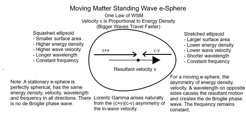
A stationary electron is a spherical, directionally equal e-sphere: it has the same \(E_d\), \(c'\), wavelength and frequency in every direction and is therefore continually rebuilt at the same place. Motion requires a three-dimensional wave egg with an elongated lower-\(E_d\) front, a flattened higher-\(E_d\) rear and a continuous side deformation. The equal frequency with unequal directional speeds produces unequal wavelengths, the internal de Broglie phase wave and the Lorentz relation.

A bound transition changes the position of the half-sphere curve imprinted on each successive background plane wave passing through the bound e-sphere. The finite sequence of changed curves carries corresponding changes of Space’s displacement, longitudinal velocity, strain and phase. A resonant receiver is progressively reshaped until it settles into another stable standing-wave mode. The propagation is continuous; the source and receiver changes are discrete because only stable recurrent organisations persist.

The electron and positron supply the two opposite radial phases; the two directions of spherical \(4\pi\) phase rotation supply the two spin states. Those four complete real-wave organisations are represented by the four Dirac sectors. Entangled pairs are source-created joint curve and phase relations; analyser settings define the available receiver modes, while the joint probabilities must reproduce Born’s rule, Bell violation and no-signalling.

“In the year nineteen hundred… the law of radiation of bodies as a function of temperature could not be derived solely from the laws of Maxwellian electrodynamics. To arrive at results consistent with the relevant experiments, radiation of a given frequency had to be treated as though it consisted of energy atoms of the individual energy (h f)… This discovery became the basis of all twentieth-century research in physics… and set science a fresh task: that of finding a new conceptual basis for all physics.”
— Albert Einstein, combined excerpts from “Considerations Concerning the Fundaments of Theoretical Physics” (1940) and “Max Planck in Memoriam” (1948)

In 1951, after half a century of work, Einstein wrote to Michele Besso:

“All these fifty years of conscious brooding have brought me no nearer to the answer to the question, ‘What are light quanta?’ Nowadays every Tom, Dick and Harry thinks he knows it, but he is mistaken.”

Glossary: Real Space, Real Waves

Claim-status key

Part I · The quantum is born

1. Planck: the furnace that would not obey classical physics

The first quantum problem was not an electron circling a nucleus. It was heat.

Imagine an enclosed cavity with a tiny opening. Its walls absorb and emit radiation until matter and light reach thermal equilibrium. The spectrum escaping the opening depends only on the temperature. At low frequencies classical reasoning worked reasonably well; at high frequencies it predicted an impossible flood of energy—the later-named ultraviolet catastrophe.

Planck modelled the matter in the cavity walls as ideal resonators of frequency \(\nu\). To reproduce the measured spectrum, he counted their energies in elements

\[ \varepsilon=h\nu, \qquad E_n=nh\nu, \qquad n=0,1,2,\ldots \]

and obtained

\[ u(\nu,T)=\frac{8\pi h\nu^3}{c^3}\frac{1}{e^{h\nu/kT}-1}. \]

Planck had introduced a new universal constant, \(h\), and a new kind of relation between energy and frequency. The quantum first entered physics through material resonators. Planck did not begin by proving that light was a shower of tiny particles moving through empty space. His calculation said that exchanges between matter and radiation occurred in frequency-linked elements.

For WSM this historical order matters. A standing-wave system naturally admits discrete mode labels because only particular phase-closing patterns remain stable. Planck’s resonators therefore point toward matter as organised wave structure. But a discrete set of allowed frequencies does not, by itself, prove discrete amplitude, discrete action or the numerical value of \(h\). The universal action unit remains a D-tier derivation.

The first lesson is nevertheless clear:

The quantum did not enter as a little object. It entered as a constraint on what a resonator could exchange.

2. Einstein: the quantum leaves the furnace

Planck had quantised the energy bookkeeping of the resonators. Einstein made the light quantum travel into the laboratory.

In 1905 he considered several phenomena that classical wave theory could not explain together, especially the photoelectric effect. When light strikes a suitable material, electrons can be emitted. Increasing the light intensity increases the number of events, but the maximum energy of an emitted electron is governed primarily by the light frequency:

\[ K_{\max}=h\nu-\Phi, \]

where \(\Phi\) is the material’s work function.

Below a threshold frequency, greater intensity does not rescue the event. Above it, energy appears in complete frequency-dependent transfers. Einstein proposed that, in emission and absorption, radiation behaved as if it were composed of localised energy quanta \(h\nu\).

This was bolder than Planck. It was also only the beginning. Einstein later analysed spontaneous emission, stimulated emission and the momentum carried in radiative exchange. The laser would eventually grow from this framework. Yet the interference of extremely weak light remained wave-like. A source can be attenuated until detector records arrive one at a time, while the accumulated pattern still depends on phase differences between alternatives.

That is the enduring puzzle. The detector record is local and complete; the wave process determining its distribution is extended and coherent.

WSM’s proposed answer begins by separating three statements that are often blended together:

1. Matter makes local, discrete records. A
2. Each complete spectral transfer obeys \(E=h\nu\). A
3. A microscopic pellet carrying that energy followed one definite path between source and detector. Not established.

In the WSM picture, a bound source is already a repeating standing-wave organisation of Space. During a transition, its changing pattern writes an ordered, finite disturbance into the travelling waves that pass through it. A resonant receiver responds to that complete wave relation and eventually recloses into a new stable state. The photon is the finite source-written curve train carried by longitudinal waves between stable source and receiver organisations; it is not a second substance or a tiny bullet independent of those waves.

This is a B/C-tier identification, not yet the final receiver-reclosure dynamics. It takes Einstein’s question literally: frequency belongs to the physical wave process, while discreteness belongs to the stable source and receiver modes.

3. Bohr: an atom that could stand still

Rutherford’s nuclear atom created an immediate crisis. In classical electrodynamics, an orbiting electron accelerates, radiates energy and spirals into the nucleus. Ordinary matter should collapse.

In 1913 Niels Bohr proposed that the atom possessed special stationary states in which this did not occur. Radiation was associated not with continuous motion around a classical orbit, but with a transition between allowed energies:

\[ E_m-E_n=h\nu_{mn}. \]

For hydrogen the model reproduced the observed spectral pattern with astonishing success. The classical orbit was still present as scaffolding, but the crucial ideas were new: stable states, discrete labels and transition frequencies.

Bohr’s “quantum jump” was a rule, not a mechanical account of how an entire atom changed. That incompleteness became one of the central tensions of quantum theory. Yet his stable-state insight survived every later formulation.

Translated into WSM language:

• a stationary state is a stable repeating standing-wave organisation of an atom;
• a spectral transition is a finite reorganisation between two such patterns;
• \(\nu_{mn}\) is the frequency of their difference relation;
• the apparatus matters because it supplies real boundary conditions and possible receiver channels.

Bohr later insisted that atomic phenomena must be described with reference to the complete experimental arrangement. That insight does not require human consciousness to create reality. Turning an analyser or inserting a which-path detector physically changes the couplings, phase relations and available records. The observer chooses the question by constructing the apparatus. The observer does not choose the answer.

4. The laboratory rebellion: atoms, recoil and divided beams

The quantum was not born from philosophy alone. Different experiments, built for different purposes, began pointing toward the same unfamiliar structure.

In 1914 James Franck and Gustav Hertz accelerated electrons through mercury vapour. The electrons surrendered energy to the atoms in sharply repeated steps rather than through an arbitrary continuum. When the mercury atoms relaxed, they emitted radiation at the corresponding spectral frequency. Bohr’s stationary states had acquired a direct collision experiment.

In 1922 Otto Stern and Walther Gerlach sent a beam of silver atoms through an inhomogeneous magnetic field. A classical distribution of tiny magnetic orientations should have spread continuously. Instead the beam divided into discrete components. The full electron-spin interpretation came later, but Nature had already displayed an irreducible two-valued response to an apparatus-defined axis.

In 1923 Arthur Compton scattered X-rays from electrons and measured an angle-dependent wavelength shift,

\[ \lambda'-\lambda=\frac{h}{m_ec}(1-\cos\theta). \]

The result joined wave frequency to directed momentum and relativistic recoil. A viable wave account of light must therefore explain not only interference and diffraction, but complete energy–momentum transfer and the Klein–Nishina angular distribution.

Then Davisson and Germer observed electron diffraction. Matter made localised detector records while its distribution was governed by extended phase. Later single-quantum double-slit and interferometer experiments sharpened the same fact: records arrive one at a time, yet the accumulated pattern depends on coherent alternatives,

\[ P=|\psi_1+\psi_2|^2 =|\psi_1|^2+|\psi_2|^2 +2\operatorname{Re}(\psi_1^*\psi_2). \]

If path information becomes physically available, the cross-term disappears. No human mind is required; the apparatus has changed the real relation.

5. De Broglie: the integers were telling us something

Louis de Broglie saw the asymmetry in the young theory. Light, long known as a wave, had acquired particle-like quanta. Matter, long treated as particles, might therefore possess wave-like phase.

His argument went deeper than analogy. A purely particle theory contained no natural frequency with which to write \(E=h\nu\). Atomic integers, meanwhile, resembled the integers found in interference and normal modes. In his Nobel lecture he emphasised precisely that clue: the earlier physical phenomena involving integers were “interference and normal modes of vibration.”

“On the one hand the quantum theory of light cannot be considered satisfactory since it defines the energy of a light particle by the equation \(E=hf\), containing the frequency \(f\). Now a purely particle theory contains nothing that enables us to define a frequency… On the other hand, determination of the stable motion of electrons in the atom introduces integers, and up to this point the only phenomena involving integers in physics were those of interference and of normal modes of vibration. This fact suggested to me the idea that electrons too could not be considered simply as particles, but that frequency must be assigned to them also.”
— Louis de Broglie, Nobel lecture (1929)

De Broglie proposed

\[ E=\hbar\omega, \qquad \mathbf p=\hbar\mathbf k, \qquad \lambda=\frac{h}{p}. \]

An electron could no longer be understood as a featureless point. Its motion carried a phase, and stable atomic states could be associated with standing-wave closure. Einstein immediately recognised the importance of the proposal. Electron diffraction, observed by Davisson and Germer in 1927, made the wavelength experimentally undeniable.

De Broglie initially retained both a particle and an accompanying wave. WSM makes the more radical identification: the matter wave is not an accessory attached to matter; the organised wave is the matter. What appears particle-like is the concentrated, repeatedly rebuilt centre of an extended standing-wave structure.

The distinction between the full Compton wavelength and its reduced form will matter later:

\[ \lambda_C=\frac{h}{mc}, \qquad \bar\lambda_C=\frac{\hbar}{mc}=\frac{\lambda_C}{2\pi}. \]

They are different phase ledgers, not interchangeable numerical conventions.

6. Heisenberg: abandon the orbit and keep the transitions

In 1925 Werner Heisenberg refused to build atomic theory from electron trajectories that no experiment could reveal. Spectroscopy gave frequencies and transition strengths, so he organised those quantities directly.

Max Born recognised that Heisenberg’s arrays obeyed matrix multiplication. With Pascual Jordan, the new matrix mechanics was developed rapidly. A physical quantity became an operator with transition elements

\[ A_{mn}=\langle m|\hat A|n\rangle. \]

Schrödinger’s continuous waves and Heisenberg’s discontinuous-looking matrices initially seemed like rival worlds. They were soon shown to be mathematically equivalent representations of the same quantum structure.

Heisenberg’s uncertainty relation followed in 1927:

\[ \Delta x\,\Delta p\geq\frac{\hbar}{2}. \]

This is often reduced to the claim that measurement disturbs a small particle. Measurement can certainly disturb a system, but the inequality is deeper. Position and momentum are Fourier-related descriptions, and their operators do not commute:

\[ [\hat x,\hat p]=i\hbar. \]

A finite wave cannot be made arbitrarily narrow in position and arbitrarily narrow in wave number at once.

In a WSM reading, Heisenberg’s matrices describe relations among stable wave patterns, not secret classical orbits hidden underneath them. The element \(A_{mn}\) is naturally read as a coupling between complete bound organisations \(n\) and \(m\). The formalism was right to place transitions at the centre of atomic physics even while remaining silent about the substance undergoing them.

7. Schrödinger: the atom begins to sing

Heisenberg had kept the observable transitions and abandoned the imagined orbit. In 1926 Erwin Schrödinger approached the same atom from de Broglie’s other direction: let it be a wave eigenproblem.

\[ i\hbar\frac{\partial\psi}{\partial t} = \left(-\frac{\hbar^2}{2m}\nabla^2+V\right)\psi, \qquad \hat H\psi_n=E_n\psi_n. \]

Boundary conditions allow only particular eigenfunctions and energies. The mysterious quantum numbers of the older atom reappeared as labels of standing-wave patterns. Hydrogen’s spectrum followed without a tiny planet circling the nucleus. Schrödinger then showed that his apparently continuous wave mechanics and Heisenberg’s apparently discontinuous matrix mechanics were equivalent representations.

This was one of the great moments in the history of thought. An abstract list of stationary states had become a geometry of modes, and two paths that looked opposed met in the same mathematics.

“Let me say at the outset that in this discourse I am opposing not a few special statements of quantum mechanics held today. I am opposing, as it were, the whole of it. I am opposing its basic views that have been shaped twenty-five years ago, when Max Born put forward his probability interpretation, which was accepted by almost everybody.”
— Erwin Schrödinger, lectures on the interpretation of quantum mechanics

Schrödinger hoped the wave was physically real and returned repeatedly to the possibility that apparent jumps arose from continuous resonance between modes. WSM keeps that instinct: discrete stable endpoints need not imply a discontinuous substance between them.

The many-body wavefunction generally lives on configuration space rather than ordinary three-dimensional space. WSM therefore reads \(\psi\) as an extraordinarily powerful collective amplitude or demodulated envelope of deeper real-space standing-wave relations—not as a second substance.

The reciprocal Doppler pair already gives a conditional route. If the solved moving e-sphere supplies

\[ \omega_{\rm ph}^2-c^2k_{\rm dB}^2=\omega_e^2, \]

write the real composite phase as

\[ \Phi_{\rm eff}=\operatorname{Re}\!\left[\psi(\mathbf x,t)e^{-i\omega_et}\right]. \]

The slow-envelope limit gives

\[ iJ_*\partial_t\psi=-\frac{J_*^2}{2m}\nabla^2\psi, \qquad m=\frac{J_*\omega_e}{c^2}, \]

which is Schrödinger’s free equation when the universal wave-action scale is \(J_*=\hbar\).

8. Pauli, Bose and Fermi: spin, exclusion and quantum identity

While de Broglie, Heisenberg and Schrödinger were rebuilding the single electron, another revolution was changing the meaning of many quanta.

In 1924 Satyendra Nath Bose derived Planck’s radiation law by counting light quanta as fundamentally indistinguishable. Einstein recognised the importance immediately and extended the method to material particles. The result predicted Bose–Einstein condensation: many integral-spin quanta may occupy one common mode.

Electrons obey the opposite rule. In 1925 Wolfgang Pauli formulated the exclusion principle: no two electrons in an atom can occupy the same complete set of quantum numbers. In 1926 Enrico Fermi and Paul Dirac developed the corresponding statistics. Exchange of two identical electrons changes the sign of the joint amplitude; two electrons cannot enter the same one-particle state.

This is why atoms possess shells, why the periodic table has its structure, why matter resists collapse and why chemistry exists. Quantum identity is not classical similarity. There is no additional hidden label saying “electron 1” and “electron 2” after the complete state has been formed.

Pauli’s other great clue was two-valuedness. Spectra and Stern–Gerlach splitting required a degree of freedom that was later recognised as electron spin. Pauli’s matrices gave its compact algebra:

\[ \sigma_x= \begin{pmatrix}0&1\\1&0\end{pmatrix}, \quad \sigma_y= \begin{pmatrix}0&-i\\i&0\end{pmatrix}, \quad \sigma_z= \begin{pmatrix}1&0\\0&-1\end{pmatrix}. \]

The spin operators are

\[ S_i=\frac{\hbar}{2}\sigma_i, \qquad \mathbf S^2=\frac34\hbar^2, \]

so any chosen axis has the two projections \(\pm\hbar/2\). A rotation through physical angle \(\theta\) is represented by

\[ U(\theta,\hat{\mathbf n}) = \exp\!\left(-\frac{i\theta}{2}\hat{\mathbf n}\!\cdot\!\boldsymbol\sigma\right), \]

which contains the half-angle, changes sign after \(2\pi\), and returns after \(4\pi\). Sequential analyser probabilities therefore contain \(\cos^2(\theta/2)\) and \(\sin^2(\theta/2)\).

Spin is not well pictured as a solid bead rotating about one little axle. A spinor transforms by a half-angle and returns to the identical complex state after \(4\pi\), while an ordinary vector closes after \(2\pi\). WSM replaces the bead with a radial standing-wave vibration carrying a spherical rotation of phase.

9. Born: the wave becomes a probability law

Schrödinger’s equation evolved amplitudes, but an experiment ended in a particular record. What connected the two?

In 1926 Max Born, studying scattering, proposed that the squared magnitude of the wave amplitude gives the probability density of an outcome:

\[ P(x)\,dx=|\psi(x)|^2dx. \]

For a projective measurement with alternatives \(|j\rangle\),

\[ P(j)=|\langle j|\psi\rangle|^2. \]

More generally, modern quantum theory writes

\[ P(j)=\operatorname{Tr}(\rho E_j), \]

where \(\rho\) is the state and \(E_j\) represents a physical measurement channel.

“Here, I would like to try to give a third interpretation and probe its utility in collision processes… I would then like to pursue the following idea heuristically… only a probability that a certain path will be followed will be determined by the function \(\psi\). One can perhaps summarize this, somewhat paradoxically, as: the motion of the particle follows the laws of probability, but the probability itself propagates in accord with causal laws.”
— Max Born, “Quantum Mechanics of Collision Processes” (1926)

Born’s rule works. It is among the most thoroughly tested rules in science. Yet it joins two different things: a continuously evolving amplitude and a discrete realised detector record. The formalism assigns their frequencies; it does not, by that fact alone, specify the microscopic process by which one receiver channel becomes the stable recorded mode.

Schrödinger objected because he wanted a real wave process. Einstein objected because he doubted that irreducible chance was the final layer of Nature. Bohr and Heisenberg emphasised that the theory concerned what could be said and measured under a complete experimental arrangement. The disagreement was not over the laboratory predictions. It was over what sort of world made them true.

WSM offers a physical location for Born’s square. Let a travelling source pattern be \(\Xi\), and let receiver channel \(j\) possess a phase-matched standing-wave mode \(D_j\). Its coherent coupling is

\[ g_j=\langle D_j,\Xi\rangle_G. \]

Here \(G\) is the positive physical action metric on the receiver-mode space after redundant phase references are removed. On the unreduced field space it may be only semidefinite, with redundant phase-reference directions in its kernel. The Action page must derive this metric once. Quantum measurement uses it for receiver work and normalization; the QED page must use the same metric for scattering flux and the optical theorem. WSM may not choose one convenient norm for Born probabilities and another for QED unitarity.

For a passive linear receiver, absorbed work is quadratic:

\[ P_{\mathrm{abs},j} = \frac{\omega}{2} \langle\Xi,\operatorname{Im}\chi_j\,\Xi\rangle \propto |g_j|^2 \]

near an isolated phase-matched receiver mode. This is an A-tier response result under its stated assumptions. It explains why a squared overlap, rather than a linear signed amplitude, belongs naturally to energy uptake.

There is also a short functional result. Let \(J_j\propto|g_j|^2\) be the action delivered to a channel, and let \(W(J)\) measure the size of its receiver-reclosure basin. If \(W\) is nonnegative, continuous and additive when one channel is refined into mutually exclusive orthogonal subchannels, then

\[ W(J_1+J_2)=W(J_1)+W(J_2) \quad\Longrightarrow\quad W(J)=\kappa J. \]

Normalisation immediately gives \(P_j=J_j/\sum_kJ_k=|g_j|^2/\sum_k|g_k|^2\). This proves the Born functional form conditional on the physical basin measure; it does not yet prove that the nonlinear detector dynamics supplies that measure. The following two-quadrature model makes one concrete route explicit.

The strongest audit is not a maximally entangled binary experiment, because nonlinear response can sometimes preserve a normalized two-channel curve while changing total efficiency. Instead refine one physical channel of action \(J\) losslessly into any number of orthogonal subchannels \(J_i\) with \(\sum_iJ_i=J\). Coarse-grained receiver probability must be unchanged:

\[ \boxed{ W(J)=\sum_iW(J_i). } \]

For example, a correction \(W(J)=J+\eta J^2\) fails because

\[ W(J)-\sum_iW(J_i) = 2\eta\sum_{i<k}J_iJ_k. \]

Lossless multiport refinement therefore tests the Born functional more severely than the singlet alone. Exact refinement invariance excludes every continuous nonlinear correction; a measured dependence on how one coherent channel is subdivided would either falsify this Born bridge or reveal non-ideal receiver dynamics.

Action, rather than raw energy, is the natural invariant currency. For a monochromatic mode

\[ J=\frac E\omega=\frac1{2\pi}\oint p\,dq. \]

Under a boost, \(E'=K_{\hat n}E\) and \(\omega'=K_{\hat n}\omega\), so \(J'=J\). Probabilities must be frame independent; WSM should therefore formulate both its sea normalization and its receiver-transition action budget in action. The invariant background target is \(J_0=\hbar/2\), not “unit energy for every observer.”

There is now a more general dynamical theorem. For exclusive branches \(\alpha\), define their normalized action shares

\[ x_\alpha=\frac{J_\alpha}{J_{\rm total}} =\frac{|M_\alpha|^2}{\sum_\beta|M_\beta|^2}, \qquad \sum_\alpha x_\alpha=1. \]

Two deductions must remain separate. The positive action metric and lossless-refinement theorem establish the initial shares \(x_\alpha(0)\propto|M_\alpha|^2\). The neutral diffusion below does not derive those initial weights; it explains how already-defined action shares can become one exclusive absorbing result without changing their ensemble means.

Reciprocal wave interference suggests antisymmetric action currents. After unresolved sea phases are coarse-grained, the minimal neutral diffusion on the action simplex is

\[ dx_\alpha=\sqrt\kappa \sum_{\beta\ne\alpha}\sqrt{x_\alpha x_\beta}\,dW_{\alpha\beta}, \qquad dW_{\beta\alpha}=-dW_{\alpha\beta}. \]

It conserves total action and has covariance and generator

\[ dx_\alpha dx_\beta =\kappa x_\alpha(\delta_{\alpha\beta}-x_\beta)d\tau, \]

\[ \mathcal L=\frac\kappa2 \sum_{\alpha,\beta}x_\alpha (\delta_{\alpha\beta}-x_\beta) \partial_\alpha\partial_\beta, \qquad \boxed{\mathcal Lx_\alpha=0.} \]

Each action share is therefore a bounded martingale. If nonlinear detector amplification reaches one exclusive absorbing vertex \(x_\alpha(\tau_c)=\delta_{\alpha R}\), optional stopping gives

\[ \boxed{ P(R=\alpha)=\mathbb E[x_\alpha(\tau_c)] =x_\alpha(0) =\frac{|M_\alpha|^2}{\sum_\beta|M_\beta|^2}. } \]

The ideal diffusion also has mean reclosure parameter

\[ \mathbb E[\tau_c] =-\frac2\kappa\sum_\alpha(1-x_\alpha)\ln(1-x_\alpha). \]

For \(N\) equally weighted branches this becomes

\[ \boxed{ T_N=\frac{2(N-1)}{\kappa}\ln\frac{N}{N-1}. } \]

In particular \(T_2=2\ln2/\kappa\) and \(T_4=6\ln(4/3)/\kappa\), so equal four-channel reclosure takes \(T_4/T_2\simeq1.2451\) times the internal reclosure parameter of equal two-channel reclosure if the same \(\kappa\) and laboratory-time map apply.

Zero drift is experimentally decisive. For two branches with a small systematic bias,

\[ dx=\epsilon x(1-x)d\tau +\sqrt{\kappa x(1-x)}\,dW, \]

the probability of absorption at \(x=1\) is

\[ \boxed{ P_1(x)=\frac{1-e^{-2\epsilon x/\kappa}} {1-e^{-2\epsilon/\kappa}} =x+\frac{\epsilon}{\kappa}x(1-x)+O(\epsilon^2). } \]

At the balanced point, a probability deviation smaller than \(\delta\) requires \(|\epsilon/\kappa|<4\delta\) to leading order. Born precision therefore directly constrains nonreciprocal drift in the proposed detector dynamics.

The fixation theorem is more general than this particular covariance. Whenever the bounded shares \(x_\alpha\) are martingales, sum to one, vanish permanently on a lost branch and eventually reach one absorbing vertex, \(P(R=\alpha)=x_\alpha(0)\). The covariance controls reclosure time and correlations along the path; the martingale plus absorption fixes the final probabilities.

The theorem is exact for the declared Itô diffusion and absorbing boundary. That convention is a physical gate, not notation. If a smooth microscopic sea first produces the same edge noise in the Stratonovich sense, conversion to Itô adds, for each pair \((i,j)\),

\[ b_i^{(ij)}=\frac{\kappa_{ij}}4(x_j-x_i), \qquad b_j^{(ij)}=-b_i^{(ij)}, \]

which preserves total action but generally destroys the individual martingales. “Chaotic background” alone therefore does not derive Born neutrality. The nonlinear Space equations must yield an impulsive or jump limit with the Itô generator, an exact compensating drift, or a reciprocal invariant measure that restores \(\mathbb E[x_\alpha]\). Its remaining WSM content is precise: derive conserved joint action, reciprocal branch currents, the correct stochastic limit, zero systematic drift and exclusive absorbing closure. The constant \(\kappa\) controls reclosure time, not the Born probabilities.

A complementary phase-space picture begins with the two real wave quadratures \(z=Q+iP\). Multiplication by \(g=x+iy\) is the real map

\[ M(g)= \begin{pmatrix} x&-y\\ y&x \end{pmatrix}, \qquad \det M=|g|^2. \]

The square is the area factor of a two-quadrature wave transformation. A reduced receiver model now makes the next step explicit.

Give each exclusive channel one unresolved canonical readiness pair

\[ z_j=\frac{Q_j+iP_j}{\sqrt2}, \qquad Y_j=|z_j|^2, \qquad \sum_jY_j=Y_*. \]

Assume that before threshold the chaotic receiver sea samples the unique rotation-invariant Liouville measure on this fixed-action shell. The action fractions then have a uniform Dirichlet distribution; equivalently,

\[ \frac{Y_j}{Y_*}=\frac{E_j}{\sum_kE_k}, \qquad E_j\ \text{independent exponential variables of equal scale}. \]

This does not insert special random detector clocks. The variables are the squared radii of one canonical \((Q,P)\) phase plane per channel.

These are reduced receiver-readiness coordinates. They do not multiply the electron’s two radial phases or two spherical spin hands and do not enter the four-state Dirac count.

Let cumulative absorbed action be

\[ A_j(u)=\kappa |g_j|^2u=\kappa w_ju. \]

Channel \(j\) reaches its separatrix when \(A_j=Y_j\). The first channel to cross is therefore

\[ j_*=\arg\min_j\frac{Y_j}{w_j} = \arg\min_j\frac{E_j}{w_j}. \]

The minimum of exponentials gives, exactly,

\[ \boxed{ \Pr(j_*=j)=\frac{w_j}{\sum_kw_k} = \frac{|g_j|^2}{\sum_k|g_k|^2}. } \]

Ties have zero measure, so one channel wins almost surely. Two real readiness coordinates are also special: one canonical phase plane gives the linear Born weight under channel refinement, whereas one or two extra pairs produce different nonlinear probability functions.

A smooth local reclosure can be represented by the fold potential

\[ V(q)=Aq^2(1-q)^2-F(t)\left(q-\frac{q^2}{2}\right), \]

where \(q=0\) and \(q=1\) label the old and new stable closures. Its old barrier disappears at the exact threshold

\[ \boxed{F_c=\frac A4}. \]

For a constant supercritical train \(F>F_c\), the reduced crossing time to the post-train separatrix \(q=1/2\) is

\[ \boxed{ T_{\min}^{(0)}(F) = \frac{ \ln2+ 3\sqrt{\frac{A}{F-A/4}} \tan^{-1}\!\left[ \frac12\sqrt{\frac{A}{F-A/4}} \right] } {\mu_q(F+2A)}. } \]

Near threshold it diverges as

\[ \boxed{ T_{\min}^{(0)} \sim \frac{2\pi} {3\mu_q\sqrt{A(F-F_c)}}. } \]

This is the saddle-node bottleneck: a train only slightly above threshold can still fail if it ends too soon. It predicts critical slowing in the reduced model and separates transition-wave energy or amplitude from train duration. The physical map from \(F,\mu_q\) to an atomic or detector timescale remains D-tier.

The all-direction version couples this collective coordinate to the receiver’s phase rings:

\[ U=V(q)+K\sum_iw_i \left[1-\cos\!\left(\theta_i-q\Delta_i\right)\right]. \]

A worked diagnostic profile

\[ \Delta(\mu)=0.55+P_2(\mu)+0.65P_4(\mu) \]

has nonzero response at the orthogonal family \(\mu=0\) and retains the \(V_4\) structure omitted by a six-axis cartoon. Its 24-ring solution crosses once and recloses all angular phases; transverse participation adds a finite rephasing delay rather than an instantaneous signal. The numerical coefficients are frozen ansatz values, not fitted constants of Nature.

If a finite matched train is too weak or too short, the receiver returns to \(q=0\). If it drives \(q\) across the separatrix, the receiver relaxes to \(q=1\). The drive is proportional to \(F(1-q)\), so that source-written train does no further work after the new mode is established at \(q=1\). A shared latch closes the losing channels. Thus the reduced model produces one crossing, one stable receiver reclosure and no repeated transfer from the same train.

This is an A-tier theorem inside a C-tier receiver ansatz. The Born/receiver-selection mechanism has been constructed conditionally; the microscopic task is to derive its canonical readiness shell, invariant mixing, fold coefficients, shared latch and outgoing energy channel from the full Space action. The old claim that a squared amplitude alone derived Born’s rule is Q-tier.

The observer has no supernatural role. A polariser, slit, screen, magnetic gradient or detector changes the physical decomposition \(\{D_j\}\). That determines which alternatives are available. It does not allow the experimenter to command which one occurs.

10. Solvay and Copenhagen: what can physics say?

At the 1927 Solvay Conference the founders confronted what they had made. The equations agreed with experiment, but the old picture of independently possessed properties had dissolved. Einstein tested the new theory with ingenious thought experiments. Bohr answered by examining the complete apparatus and showing that different experimental arrangements make different complementary quantities definite.

“Copenhagen” was never one perfectly uniform creed. Born supplied the probability rule. Heisenberg emphasised uncertainty, potentiality and state reduction. Bohr emphasised complementarity and the indivisibility of the phenomenon from the conditions under which it is recorded. Later textbooks often condensed this plurality into a recipe: prepare a state, evolve it, choose an observable, apply Born’s rule and update the state after a result.

The sophistication is important. Bohr was not saying that a human gaze magically manufactures an atom. He was saying that position, momentum, path and polarisation are not context-free labels read by an apparatus that leaves their meaning unchanged. The apparatus is part of the physical phenomenon.

Einstein accepted the predictions and rejected the elevation of the probability algorithm into a complete ontology:

“I cannot but confess that I attach only a transitory importance to this interpretation. I still believe in the possibility of a model of reality—that is to say, of a theory which represents things themselves and not merely the probability of their occurrence. On the other hand, it seems to me certain that we must give up the idea of complete localization of the particle in a theoretical model.”
— Albert Einstein, Herbert Spencer Lecture (1933), published as “On the Method of Theoretical Physics” (1934)

WSM accepts the contextual lesson while rejecting the need for an unknowable substrate. A slit, polariser or magnet changes the real mode decomposition and receiver boundary conditions. The physical question changes. One Vibrating Space continues to exist and move throughout the experiment.

11. Von Neumann, mixtures, decoherence and one actual record

John von Neumann gave quantum theory its rigorous state-and-measurement architecture. Pure states are rays in Hilbert space; observables are operators; statistical mixtures are density matrices; composite systems use tensor products; ideal outcomes are represented by projections. Modern measurements generalise the projectors to positive operators \(E_j\), giving

\[ P(j)=\operatorname{Tr}(\rho E_j). \]

This language answers an essential question that ordinary words blur. A coherent alternative is not the same thing as ignorance about a fixed alternative. For the two photon modes \(|HV\rangle\) and \(|VH\rangle\), compare

\[ \rho_{\rm ent}=|\Psi^-\rangle\langle\Psi^-|, \qquad |\Psi^-\rangle=\frac{|HV\rangle-|VH\rangle}{\sqrt2}, \]

with the classical mixture

\[ \rho_{\rm mix}=\frac12|HV\rangle\langle HV| +\frac12|VH\rangle\langle VH|. \]

The entangled state contains off-diagonal phase relations; the mixture does not. Interference and rotated-basis coincidence experiments distinguish them. Yet either wing of the singlet alone has the reduced state

\[ \rho_A=\rho_B=\frac I2. \]

The whole relation is pure while each local description is maximally mixed. This is the mathematical heart of entanglement.

Measurement then exposes the famous dual structure. Between records, the quantum state evolves linearly and unitarily. At a record, the textbook state is conditioned on one outcome. Decoherence explains much of the intervening physics: the apparatus becomes entangled with an enormous environment, relative phases between macroscopically distinct records become inaccessible, and a stable pointer basis emerges. It explains why alternatives cease to interfere in practice. It does not, by itself, say why this experiment contains one actual record rather than the unobserved sum of all records.

“In the case of the waves of wave mechanics we have no idea what is waving… and do not ask the question… There is no hint in the mathematics that the actual phenomenon is a minute flash at some particular point… It is only in applying the rule, relating the probable location of the flash to the intensity of the wave, that indeterminism enters the theory.”
— John S. Bell, “Six Possible Worlds of Quantum Mechanics”

WSM supplies a visual candidate for the missing physical step. The state vector is the modal ledger of real wave relations; decoherence is differential phase scrambling into uncontrolled e-spheres; each detector channel is a possible stable standing-wave mode. Incoming curves deform several possible modes, the nonlinear threshold leaves one stable receiver reclosure, and that reclosure is the persistent record. The Haar–Liouville readiness-shell and fold models in §9 calculate normalized Born frequencies and one receiver channel inside their declared ansatz. The Space action must produce that mechanism from the real waves.

Part I continued · The unfinished argument about reality

12. Einstein, Podolsky and Rosen: is the wavefunction complete?

By 1935 quantum mechanics was already powerful. Einstein, Boris Podolsky and Nathan Rosen asked whether it was complete.

Their original thought experiment concerned two systems prepared with correlated position and momentum. After separation, a measurement on one side allows a corresponding property of the other to be predicted. If the distant measurement cannot physically disturb the remote system, EPR argued, then the remote property must already be an element of reality. Quantum mechanics did not assign simultaneous sharp values to both quantities, so they concluded that its description was incomplete.

Schrödinger responded that year by naming the central feature entanglement. The state of the whole may be definite while neither part has its own independent pure state. This was not a small correction to classical probability. It was a new kind of composition.

The later Bohm spin version makes the issue transparent. A pair is prepared in the singlet relation

\[ |\Psi^-\rangle = \frac{|+\rangle_A|-\rangle_B-|-\rangle_A|+\rangle_B}{\sqrt2}. \]

If both analysers are aligned, the outcomes are always opposite, yet each local outcome is individually random. The same perfect anticorrelation holds for every common axis. This cannot be represented as two particles carrying one unknown but fixed ordinary direction: rotating both analysers away from that direction would destroy perfect anticorrelation.

EPR did not discover a faster-than-light message. They exposed a dilemma about separability, locality and completeness.

13. Bohm: reality returns, but locality does not

David Bohm transformed the debate twice. He recast EPR in terms of two-valued spin measurements, giving the form later used by Bell. Then, in 1952, he constructed an explicitly causal and deterministic interpretation of nonrelativistic quantum mechanics.

In Bohm’s theory, particles have positions and are guided by a real wavefunction. The theory reproduces ordinary quantum predictions, but the guiding law for many particles is nonlocal: the configuration of the whole enters the motion of each part.

This was historically decisive. It showed that quantum statistics did not logically force the abandonment of objective reality or determinism. It also showed the price of retaining them in that form: nonlocality was already present.

“But in 1952 I saw the impossible done. It was in papers by David Bohm. Bohm showed explicitly how parameters could indeed be introduced… with the help of which the indeterministic description could be transformed into a deterministic one. More importantly, in my opinion, the subjectivity of the orthodox version, the necessary reference to the ‘observer,’ could be eliminated.”
— John S. Bell, “On the Impossible Pilot Wave” (1982)

“Why is the pilot wave picture ignored in text books? Should it not be taught… to show that vagueness, subjectivity, and indeterminism are not forced on us by experimental facts, but by deliberate theoretical choice?”
— John S. Bell (1982)

Bohm later spoke of wholeness and the danger of treating the world as independently existing fragments. WSM shares that relational instinct but proposes a different ontology. It seeks to remove the remaining point particles and the fundamental configuration-space wave, replacing both with finite centres and extended relations of one real Space.

“The notion that all these fragments are separately existent is evidently an illusion.”
— David Bohm, Wholeness and the Implicate Order (1980)

That ambition raises a harder question than simply declaring everything connected. Can a real-space wave theory reproduce the exact nonlocal correlations without reducing them to local hidden instructions?

John Bell supplied the test.

14. Bell: the line Nature crossed

Bell’s 1964 theorem did not say that every realistic theory was impossible. Bohm’s model was already a counterexample. Bell showed that a broad class of locally causal completions cannot reproduce all quantum predictions.

If a common cause \(\lambda\) is distributed independently of later settings \(\mathbf a,\mathbf b\), and each outcome depends only on its local setting and relevant past data, the joint probability factorises:

\[ P(r,s|\mathbf a,\mathbf b) = \int d\lambda\,\rho(\lambda) P_A(r|\mathbf a,\lambda) P_B(s|\mathbf b,\lambda). \]

This structure implies a Clauser–Horne–Shimony–Holt bound

\[ |S|\leq2. \]

For a spin singlet, quantum theory predicts

\[ P(r,s|\mathbf a,\mathbf b) = \frac14\left(1-rs\,\mathbf a\cdot\mathbf b\right), \]

\[ E(\mathbf a,\mathbf b) = \sum_{r,s=\pm1}rs\,P(r,s|\mathbf a,\mathbf b) = -\mathbf a\cdot\mathbf b, \]

and suitable settings give

\[ |S|=2\sqrt2. \]

For photon polarisation, physical analyser angles are represented by doubled angles on the Bloch sphere, yielding correlations of the form

\[ E(\alpha,\beta)=\pm\cos 2(\alpha-\beta), \]

with the sign fixed by the prepared Bell state.

Bell’s bound is not a generic “straight line” that quantum theory bends. It follows from a precise causal factorisation. Shared ancient waves, local conservation laws, common classical orientations and two independent detector races all remain Bell-bounded if they enter only through \(\lambda\) and local response functions.

Experiments violate Bell inequalities while preserving random local marginals. What they exclude is a setting-independent table of local answers carried from the source, under the ordinary independence assumptions. They do not by themselves prove consciousness, controllable faster-than-light signalling, irreducible randomness or the literal splitting of worlds.

Bell made the reality question experimental.

15. What the laboratories actually create

The phrase “two entangled particles” can hide the most important physical fact: the preparation creates one coherent relation with two separated ends.

Entangled photons

A common modern source uses spontaneous parametric down-conversion. A pump wave enters a nonlinear crystal. With low probability, the crystal transfers one pump-frequency excitation into a signal–idler pair of allowed modes. Energy and phase matching constrain the whole creation process:

\[ \omega_p=\omega_s+\omega_i, \qquad \mathbf k_p\approx\mathbf k_s+\mathbf k_i, \]

with the finite crystal supplying a calculable phase-matching width rather than an infinitely sharp equality.

The corresponding classical three-wave action balance is the Manley–Rowe relation

\[ -\dot J_p=\dot J_s=\dot J_i. \]

Thus one complete conversion has \(\Delta J_p=-\hbar\) and \(\Delta J_s=\Delta J_i=+\hbar\), while \(\omega_p=\omega_s+\omega_i\) preserves energy. The pair is one coherently created bilocal relation, but a successful pair measurement contains two endpoint absorptions. Exclusivity means that only one joint channel pair \((r,s)\) completes—not that one quantum of action is divided between two detectors.

Entanglement is created when two or more alternatives are made coherent and no physical record distinguishes them. A polarisation source may prepare, ideally,

\[ |\Psi^-\rangle = \frac{|H\rangle_A|V\rangle_B-|V\rangle_A|H\rangle_B}{\sqrt2}. \]

This is not a statistical mixture in which one photon was secretly horizontal and the other secretly vertical. The relative phase between the two creation alternatives is experimentally active. Change it, preserve it or destroy it, and the later coincidence table changes.

The source can be written without picturing two pre-labelled pellets. Let \(G^T\) be the transverse response from a creation point \(z\) to the two output regions and let \(\chi^{(2)}\) be the crystal’s nonlinear response. The pair kernel has the form

\[ \Xi_{ij}(x_A,x_B) = \int d^4z\, G^T_{im}(x_A,z) G^T_{jn}(x_B,z) \chi^{(2)}_{pmn}(z)\,\mathcal E_p(z). \]

Projection onto the two allowed polarisations at each end gives the \(2\times2\) source matrix

\[ C_{\lambda\mu} = \epsilon_{\lambda}^{i*}\, \Xi_{ij}\, \epsilon_{\mu}^{j*}. \]

A pure two-polarisation pair is separable exactly when this matrix has rank one; it is entangled when its rank exceeds one—equivalently, for a nonzero \(2\times2\) pair, when \(\det C\neq0\). The antisymmetric Bell source is represented by

\[ C=\frac1{\sqrt2} \begin{pmatrix} 0&1\\ -1&0 \end{pmatrix}. \]

For analyser vectors \(u_+(a)=(\cos a,\sin a)\) and \(u_-(a)=(-\sin a,\cos a)\), the joint amplitude is \(M_{rs}=u_r(a)^TCu_s(b)\). Born weighting gives

\[ P_{++}=P_{--}=\frac12\sin^2(a-b), \qquad P_{+-}=P_{-+}=\frac12\cos^2(a-b), \]

and therefore \(E(a,b)=-\cos2(a-b)\). This calculation identifies exactly what is connected: the coherent source tensor and its two endpoint projections. Experiments that spectrally resolve SPDC identify imbalance between the two decay paths as a direct cause of reduced polarisation-entanglement quality.

At each wing, wave plates and a polarising beam splitter define a measurement basis. The two output ports feed detectors. The apparatus records a setting, an output label and a time tag. Only after the two local records are compared are paired trials identified and the four joint frequencies estimated:

\[ P(++|a,b),\quad P(+-|a,b),\quad P(-+|a,b),\quad P(--|a,b). \]

Quantum-optical controls probe the detector-response structure itself. An ideal single-photon source sent to two outputs is antibunched, with \(g^{(2)}(0)=0\): one prepared excitation does not become two simultaneous complete detections. Conversely, two indistinguishable photons arriving at a balanced beam splitter show Hong–Ou–Mandel interference and leave together. These are not decorative paradoxes; they test exclusivity, indistinguishability and coherent two-mode addition.

No isolated click displays “nonlocality.” The nonlocal fact is the setting-dependent structure of this joint table together with the impossibility of decomposing it into Bell’s local form.

Entangled electrons

Electron spins can be entangled through interactions that conserve total angular momentum, through exchange coupling in neighbouring quantum systems, or by entanglement swapping. In a landmark loophole-free experiment, remote electron spins associated with diamond defects were first entangled with emitted photons. Interference and a heralding detection then projected the distant electron spins into one entangled relation. Each spin was read locally using a separately chosen basis.

The physical implementation differs from a photon polariser, but the logical measurement is the same: prepare a pair relation, choose two local decompositions, produce two records, and test their joint statistics.

For massive particles, a Stern–Gerlach magnetic gradient is the historical model of a spin analyser. Modern electron-spin experiments often rotate the spin with microwave pulses and convert its state into a local fluorescence or charge record. “Spin up” never means absolutely up. It means the output channel selected relative to the physical analyser axis used in that trial.

The experimental arc

Freedman and Clauser observed a Bell-inequality violation with photons in 1972. Aspect, Dalibard and Roger changed analyser conditions during the photons’ flight in 1982. In 2015 independent experiments closed the principal detection and locality loopholes in the same test. In 2017 entangled photons distributed from the Micius satellite violated a Bell inequality across roughly 1,200 kilometres.

The experiments do not show that one detector sends a readable instruction to the other. The ideal maximally entangled law has fair random local marginals:

\[ P(r|\mathbf a,\mathbf b)=\frac12, \qquad P(s|\mathbf a,\mathbf b)=\frac12. \]

The remote setting changes no controllable local frequency. The correlation appears only when records are later compared through ordinary communication.

This is what any WSM account must explain: not a mystical influence visible at one detector, but one relation that produces two local records and refuses local factorisation.

16. Were the two outcomes genuinely open—or merely unknown?

The usual alternatives are often stated too crudely.

If “fixed” means that each member carried a local answer for every possible analyser direction, Bell experiments exclude that model under measurement independence. If “open” means that nothing physical existed until a conscious person looked, the experiments do not establish that either.

Kochen–Specker contextuality sharpens the point even without a distant partner: quantum observables cannot all possess one noncontextual table of predetermined values that preserves their required relations across every compatible measurement arrangement. This does not abolish reality. It says the actual property belongs to the real system–apparatus relation, not to an isolated object carrying answers to every unperformed question.

A more precise possibility is contextual realism:

• the source prepares a real invariant relation, not two complete answer tables;
• the analysers physically define the channels available in the chosen bases;
• those channels are genuine possible receiver-reclosure modes;
• one joint receiver branch becomes the actual pair of records;
• consciousness neither creates the channels nor chooses the branch.

Two causal versions remain possible. The complete global wave state and boundary data may select the branch deterministically, while no outcome was locally preassigned for unrealised settings. Or nonlinear receiver reclosure may contain irreducible stochasticity. Bell tests distinguish neither. They constrain the causal structure, not every possible ontology beneath it.

The measurement setting determines which physical question is implemented. It does not determine which answer the experimenter receives.

Part II

One Vibrating Space

Real longitudinal compression waves

“Physical objects are not in space, but these objects are spatially extended. In this way the concept ‘empty space’ loses its meaning.”
— Albert Einstein, note dated 9 June 1952 to the fifteenth edition of Relativity: The Special and the General Theory

Space is the one physical substance and is therefore necessarily infinite, eternal and continuous. It is nearly rigid and slightly elastic. Its regions remain connected to their neighbouring regions and vibrate backwards and forwards through small distances. A compression travels because each region compresses the next region and then returns towards its balanced position.

We represent this real motion with longitudinal plane waves travelling in every direction. A plane wave has a flat plane of equal phase. The compression advances at right angles to that plane, and Space vibrates backwards and forwards in exactly the same direction that the wave travels:

The complete motion is the overlap of these waves over every direction:

Every term is a vibration of the same Space. The enduring connection of neighbouring regions makes Space solid in the ontological sense. Ordinary material solids are later structures made from bound e-spheres; their atomistic shear modes do not define the primitive vibration of Space.

How all-direction plane waves form an e-sphere

An electron is an open, stable, spherical standing-wave organisation formed where longitudinal plane waves from every direction continually interact. The waves converge towards the wave centre, cross the centre and continue. A wave approaching from one side becomes a wave receding on the other side because it has passed through the centre; it remains the same longitudinal compression wave.

The Huygens sphere is the boundary condition for the e-sphere. Through this finite spherical relation, the surrounding background plane waves set the incoming phase, energy-density and recurrence conditions under which the e-sphere continually re-forms. The waves cross the centre and continue while the Huygens-sphere relation maintains the complete coherent boundary condition.

The equal all-direction phase sum gives

The spherical compression and extension can be written

with its linked quarter-cycle longitudinal motion

At maximum compression or extension, the local velocity is zero. A quarter-cycle later, the regions of Space pass through their balanced positions with maximum radial velocity. Another quarter-cycle reverses the compression. These are successive phases of one real spherical vibration.

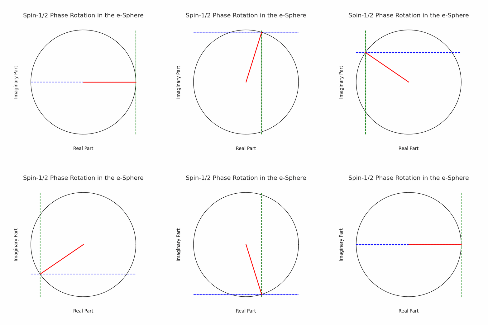
Why the spherical e-sphere remains stationary

A stationary e-sphere is spherical. At a given radius its directional wave-energy density \(E_d\) is therefore the same in every direction. The One Law

then gives the same local propagation speed \(c'\) in every direction. Resonant stability requires one common frequency \(f_e\) throughout the complete e-sphere. Since

equal \(c'\) and equal frequency give equal wavelength in every direction:

Every directional wave returns to the same phase relation at the same centre. Every directional change is balanced by the corresponding change from the opposite direction. Successive waves therefore rebuild the e-sphere at the same position in Space. Its spherical equality is the physical cause of its stationary centre.

A The \(j_0/j_1\) all-direction identities are exact. B The stationary e-sphere is their WSM physical interpretation.

Matter, antimatter and universal clocks

Opposite radial phase

An electron and positron are the same kind of spherical standing-wave organisation held in opposite phase relative to the background plane waves:

When the electron pattern is compressing, the positron pattern is stretching. When regions of Space in the electron recurrence move radially inward, the corresponding regions in the positron recurrence move radially outward. Half a cycle later both motions have reversed while their opposition remains.

The phase difference is physical because both e-spheres are continually measured against and maintained by the same background sea of plane waves. It is a relation between complete physical wave organisations, not an arbitrary sign attached to an isolated symbol.

Frequency locking and the cosmic clock

The common background locks electron and positron to the same rest frequency \(\omega_e\). They therefore possess the same positive rest energy and mass while remaining opposite radial-phase organisations.

This stable frequency is necessary for existence. Plane waves arriving from every direction must remain phase-locked if they are to meet, cross and reproduce one e-sphere after every cycle. A drift among their frequencies would destroy the common spherical recurrence.

Every free electron therefore carries the same resonantly selected rest-frequency clock. Atomic clocks ultimately compare stable recurrences made from these same e-spheres. Motion changes the directional wavelengths and the rate at which the complete recurrence is observed, while the resonant identity of the e-sphere remains fixed.

B Opposite background-relative radial phase is the WSM electron–positron identification.

Spin is a spherical rotating phase wave

The complete sphere rotates in phase

The radial compression is not the complete electron. Plane waves arriving from different directions overlap throughout the whole spherical region. Their equal-phase intersections form a second pattern: a phase wave that rotates spherically through the complete e-sphere.

This is spherical rotation. The phase relation changes throughout the entire three-dimensional sphere. Every direction participates. Each underlying compression wave continues travelling longitudinally; the spherical rotation is the changing three-dimensional pattern created by their overlap.

The spherical phase wave can progress faster than the longitudinal compression waves because it is the movement of a phase intersection. The causal motion of each region of Space and the transport of every new change remain carried by the longitudinal waves at \(c'\).

Two opposite spherical rotations

The spherical phase sequence has two possible directions:

They may be represented by

Changing \(h\) reverses the complete spherical phase sequence while leaving the electron or positron radial phase unchanged. These are the two physical spin states. When a measuring apparatus establishes an axis, it resolves the two spherical rotations as the two observed projections conventionally called spin up and spin down.

The first-order hand fields

The radial compression and spherical phase order can be joined as

The spherical Bessel identities give

The two spherical hands are therefore exact eigensectors of a first-order spatial operator. Squaring the operator returns the second-order Helmholtz wave equation. The Pauli-type first-order structure is already present in the all-direction wave geometry.

Why the wave returns after \(4\pi\)

After one \(2\pi\) spherical rotation, the ordinary spatial orientation has returned but the complete chronological phase relation has reached its opposite endpoint:

A second \(2\pi\) transformation restores both spatial orientation and chronological phase:

The mathematical lift is

Battey-Pratt and Racey developed this spherical-rotation geometry and related it to the Dirac equation. WSM gives this geometry a physical realisation in the ordered intersections of longitudinal plane waves overlapping throughout a complete spherical standing wave.

If the nonlinear Space action yields the e-sphere wave action \(J_*=\hbar\), the rotation generator is

A The \(SU(2)\), Pauli and \(4\pi\) geometry is exact. B WSM identifies it with the spherical phase wave of the e-sphere.

The real-wave foundation of the Dirac equation

The WSM electron postulate. An electron is a spherical e-sphere recurrence formed from longitudinal background plane waves converging from every direction, crossing the centre and continuing outward. Its \(j_0\) compression pattern and quarter-cycle \(j_1\) motion form one complete spherical vibration. The opposite background-relative radial phase forms the positron. Each radial phase admits two opposite spherical \(4\pi\) rotations. These four real-wave states are represented by the four Dirac sectors. The remaining action-equation problem is to prove their nonlinear stability and calculate their physical properties.

Four real-wave Dirac states

The e-sphere has two independent physical binary relations:

1. two opposite radial phases relative to the background, \(q=+1\) and \(q=-1\);
2. two opposite directions of spherical phase rotation, \(h=+1\) and \(h=-1\).

How the four real-wave states carry the Dirac factorisation

Let the Pauli matrices \(\tau_i\) act on the two background-relative radial phases, and let \(\sigma_i\) act on the two spherical rotation hands. The coordinate space of the four complete e-sphere states is therefore

The explicit bridge to Dirac’s matrices is

Consequently the minimal isotropic first-order generator that joins propagation, spherical hand and the opposed rest-phase recurrence is

Thus two radial phases multiplied by two spherical hands supply the minimal four-dimensional representation required by the Dirac–Clifford factorisation. The mass matrix distinguishes the opposite radial phases; the propagation matrices join their transformation to the two spherical hands.

Why the notation is complex

Every one of the four solutions is a real spherical vibration with a compression pattern and a velocity pattern. Two real numbers record its amplitude and its position within the vibration cycle:

The mathematical \(i\) records a real quarter-cycle phase relation. In a rest basis organised by radial phase and spherical rotation, the four-component spinor is the coordinate ledger

A moving or interacting e-sphere is one complete changing pattern whose mathematical coordinates mix. The four entries name possible complete wave organisations, not pieces from which an electron is assembled.

A real first-order wave factorisation

A one-dimensional slice through the all-direction recurrence makes the first-order algebra visible. Let \(a_{\rightarrow}\) and \(a_{\leftarrow}\) record the real compression and quarter-cycle motion of the longitudinal wave relations travelling in the two opposed directions along that slice. Let \(\mathsf J\) be the real ninety-degree operation between those two phases, with \(\mathsf J^2=-I\). Then

Applying either first-order operator twice gives

With \(E=\hbar\omega\), \(p=\hbar k\) and \(mc_0^2=\hbar\omega_e\), this is

The opposed arrows name propagation directions within one real spherical vibration; they are not “reciprocal reconstruction grades” and do not multiply the four physical states. The full three-dimensional factorisation replaces the one-axis sign by the Pauli–Clifford spherical rotation algebra.

What the Dirac operator describes

The equation joins three real processes:

• the continuing rest-frequency compression and extension of the e-sphere;
• the changing directional phases of the longitudinal plane waves when the e-sphere moves;
• the two spherical rotations of the phase-intersection pattern.

The Pauli matrices represent the spherical rotation algebra. The spatial Dirac matrices describe how radial phase and spherical rotation transform together under motion. The rest term records the stable recurrence frequency and distinguishes the opposed electron and positron radial phases:

The Clifford anticommutation relations ensure that squaring the first-order equation returns

A Dirac factorisation and its experimental consequences are established. B/C The four real-wave solutions and spherical phase anatomy supply the WSM foundation.

Motion: the spherical e-sphere becomes a wave egg

Spherical equality fixes the resting centre

An exactly spherical e-sphere cannot translate while its directional wave conditions remain identical. Equal \(E_d\), equal \(c'\), equal wavelength and equal frequency continually rebuild the same spherical centre. Translation requires a three-dimensional directional asymmetry.

The moving wave egg

A moving e-sphere is rebuilt as an egg-shaped standing-wave organisation:

The sides also stretch and reshape, completing one three-dimensional egg. The common frequency remains

That frequency equality is a condition of resonant stability. Directional frequency drift would make the arriving phases lose their common recurrence. With \(f_e\) fixed, the One Law makes the directional speed change appear as a directional wavelength change:

De Broglie phase and the Lorentz factor

The front and rear waves retain the same frequency while their speeds and wavelengths differ. In the canonical opposed-wave picture,

The unequal wavelengths have unequal wave numbers,

The changing phase difference between these opposed waves creates the internal de Broglie phase wave. Their speed product contains the Lorentz factor:

The same front–rear wavelengths give the exact ratio

For the hydrogen ground-state identification \(v=\alpha c_0\), this ratio is approximately \(1.01470\): the rear wavelength is about \(1.47\%\) longer than the leading wavelength. Relative to the undeformed reference \(\lambda_0=c_0/f_e\), the rear is \(+\alpha\approx+0.730\%\) and the lead is \(-\alpha\approx-0.730\%\). This is a concrete wave-egg target for the nonlinear solution.

The e-sphere centre moves because successive all-direction interactions reconstruct the wave centre at successive positions. The de Broglie phase wave can be superluminal because it is the progression of a phase relation; the changing Space and transported energy remain causal.

Frequency dictionary for the moving e-sphere

The common \(f_e\) above names the one intrinsic recurrence frequency locked through every direction of the complete wave egg. It must not be confused with the two laboratory Fourier frequencies obtained when that moving recurrence is decomposed into opposed travelling waves. With \(\omega_e=2\pi f_e\), \(k_e=\omega_e/c_0\) and \(\beta=v/c_0\), those laboratory frequencies are

The common-frequency egg relations describe directional reconstruction within Space; the Doppler pair describes the same recurrence in laboratory Fourier coordinates. They agree on the reciprocal front–rear ratio, but the laboratory \(\omega_\pm\) are not the direction-locked internal \(2\pi f_e\).

The same boosted standing-wave relation can be displayed as

The first factor reconstructs an envelope moving at \(v\). The second is the internal de Broglie phase relation with

At the moving centre \(x=vt\), its phase advances as \(\omega_e t/\gamma\), which is the Lorentz-slowed laboratory reading of the same intrinsic e-sphere clock. The intrinsic recurrence, the two travelling-wave frequencies and the laboratory clock rate are therefore distinct quantities.

The Schrödinger limit

At speeds small compared with \(c\), remove the rapid rest-frequency recurrence and retain the slowly changing de Broglie envelope. With \(mc^2=\hbar\omega_e\), the envelope obeys the free Schrödinger equation:

The wavefunction records the phase and amplitude of the extended moving e-sphere and its possible relations to other standing-wave structures.

A The constant-frequency speed product gives the Lorentz factor exactly under the stated front–rear relations. B/C The moving egg supplies the physical phase geometry.

Part III

Light: changing half-sphere curves on real plane waves

A stable bound state repeats one curve pattern

Atoms are bound standing-wave organisations of e-spheres. As a background plane wave crosses a bound e-sphere, the directional change in \(E_d\) changes \(c'\), crossing time, wavelength and phase. The plane wavefront leaves with a real half-sphere curve imprinted upon it.

In a stable bound state, successive plane waves receive the same half-sphere curve in the same repeating position. The complete bound structure therefore reconstructs the same mode cycle after cycle.

A transition moves the curve on successive wavefronts

When the bound structure changes from one stable mode to another, it changes the position of the half-sphere curve imprinted on each successive plane wave passing through it.

The first wavefront receives the curve in the old position. The next receives it slightly displaced. Further wavefronts carry the ordered sequence until the new stable atomic pattern is established. This finite sequence of changing half-sphere curves is the emitted light train.

Because each curve is a real deformation of Space, its changing position on successive plane waves carries a corresponding change in:

• the displacement of Space on the wavefront;
• the velocity of that displacement;
• the compression and extension of neighbouring Space;
• the wavelength and phase;
• the energy and wave action of the whole train.

One photon

A photon is one finite train of changing curves written during one complete bound-state transition. When its frequency, phase and curves match an allowed receiver mode, the train can rebuild that receiver into the corresponding stable standing-wave organisation.

Its frequency is the repetition rate of the curve pattern. Its energy is

when the complete train carries the universal wave-action unit. A free e-sphere continually repeats its stable curve pattern and does not emit a discrete train merely by existing. Radiation is written when a bound relationship changes.

Two photon helicities from longitudinal waves

The individual plane waves carrying the train remain longitudinal compression waves. Across the complete directional collection, the curve and phase pattern can change around the propagation direction in either of two handed orders. These are the two photon helicities:

The first angular harmonic on the Huygens ring supplies exactly those two hands. Its transverse geometry describes the arrangement of curves across many longitudinal plane waves; the vibration of every individual plane-wave component remains longitudinal.

Maxwell’s fields as organised curve relations

Take the two real transverse moments of the travelling curve pattern as \(\mathbf X\) and \(\mathbf Y\). They are the two independent first-moment components of the changing half-sphere curve across the Huygens ring, not added substances or primitive transverse vibrations of Space. Locality, isotropy, opposite parity and positive wave energy select the paired evolution

These are Maxwell’s free-wave equations after identifying the two moments with the electric and magnetic field description. The field vectors record the changing geometry of one real train carried by the waves of Space.

A The two ring harmonics and Maxwell algebra are exact inside the stated directional construction. B/C The changing half-sphere train is their real-wave interpretation.

Exact and conditional construction

Directional phase, two light hands and Maxwell geometry

Each symbol in this section refers to the curve, timing or phase relations written on real longitudinal plane waves. The individual waves continue to move Space backwards and forwards in their own directions of travel. The scalar-plus-vector connection, electric and magnetic fields and two helicities describe the collective relation among many such directions. Tier A marks the exact angular and field mathematics; tiers C and D mark the task of deriving its physical coefficients from the nonlinear Space action.

Two photon helicities from collective longitudinal Space waves

The two observed photon helicities are not transverse vibrations of individual Space waves. The light train is collective: every constituent Space wave remains longitudinal along its own direction, while the all-direction phase and curve relation contains the two transverse geometrical hands resolved by an analyser.

Let \(a(x,\hat{\mathbf n})\) denote a small phase-reference or curve perturbation associated with the Space waves arriving from direction \(\hat{\mathbf n}\). Its four-dimensional coherent sector can be identified both by scalar and vector angular moments and, more strongly, by local phase additivity.

It need not be selected merely by inspection. Let \(\alpha_x(v)\) be the phase increment assigned at \(x\) to an infinitesimal displacement \(v\). If local phase transport is continuous, additive and homogeneous,

\[ \alpha_x(v+w)=\alpha_x(v)+\alpha_x(w), \qquad \alpha_x(\lambda v)=\lambda\alpha_x(v), \]

then it is a spacetime one-form: \(\alpha_x(v)=A_\mu(x)v^\mu\). Restrict it to the future-null directions \(\ell_{\hat n}^{\mu}=(1,\hat{\mathbf n})\):

\[ \boxed{ a_{\hat n}=A_\mu\ell_{\hat n}^{\mu} =A_0+\hat{\mathbf n}\cdot\mathbf A. } \]

Thus local additive phase implies a spacetime one-form and hence exactly \(l=0\oplus1\) directional content. Higher harmonics describe finite-path curvature, multipolar sea distortion or internal e-sphere deformation rather than extra electromagnetic components. This is exact mathematics conditional on the additive local-phase premise; the Space action must still make that premise physical.

The connection also fits WSM’s existing Doppler geometry. Under a Lorentz boost a null direction transforms projectively as

\[ \Lambda\ell_{\hat n}=K_{\hat n}\ell_{\hat n'}, \qquad K_{\hat n}=W-P\,\hat{\mathbf n}\cdot\hat{\mathbf v} =\gamma(1-\boldsymbol\beta\cdot\hat{\mathbf n}), \]

with \(a'_{\hat n'}=K_{\hat n}^{-1}a_{\hat n}\) and aberration measure \(d\Omega'=K_{\hat n}^{-2}d\Omega\). The coefficients transform as a Lorentz four-potential one-form—or, after raising the index, as a four-vector. The same reciprocal identity \(W^2-P^2=1\) that generated the Lorentz–de Broglie factor now supplies a Lorentz-covariant Huygens connection.

\[ A_0(x)=\frac1{4\pi}\int_{S^2}a(x,\hat{\mathbf n})\,d\Omega, \qquad \mathbf A(x)=\frac3{4\pi}\int_{S^2}\hat{\mathbf n}\,a(x,\hat{\mathbf n})\,d\Omega. \]

The corresponding \(l=0\oplus l=1\) projection is \((P_{01}a)(\hat{\mathbf n})=A_0+\hat{\mathbf n}\cdot\mathbf A\). Orthogonality of spherical harmonics gives the exact positive complement

\[ \boxed{ Q_{01}[a] =\frac{\mu_*^2}{2} \left[ \int a^2d\Omega -\frac1{4\pi}\left(\int a\,d\Omega\right)^2 -\frac3{4\pi}\left|\int\hat{\mathbf n}a\,d\Omega\right|^2 \right]\ge0. } \]

Equality holds exactly for \(a=A_0+\hat{\mathbf n}\cdot\mathbf A\). Thus a scalar directional field possesses a natural four-dimensional coherent sector and a positive residual measuring everything that cannot be represented by one scalar plus one ordinary vector. A local angular operator with the same kernel is

\[ K_\Omega=\Lambda^2L^2(L^2-2), \qquad L^2=-\Delta_{S^2}, \]

whose eigenvalues vanish for \(l=0,1\) and are positive for \(l\ge2\). The projector and operator are exact mathematics; identifying either as the Hessian of Vibrating Space is a C-tier action ansatz.

The ordinary spherical-harmonic projector \(P_{01}\) is orthogonal in the chosen e-sphere or sea rest frame. It does not commute with boosts on an arbitrary directional field: aberration can move higher harmonics into lower spherical moments. What is Lorentz closed is the additive connection sector itself, because \(a'_{\hat n'}=K_{\hat n}^{-1}a_{\hat n}\) preserves the one-form relation. Thus the connection is covariant, while an arbitrary split \(a=P_{01}a+(I-P_{01})a\) is not automatically observer independent.

A covariant angular-content diagnostic is the trace-free spherical Hessian

\[ \mathcal S_{AB}[a] =\left(\nabla_A\nabla_Ba\right)^{\rm TF}, \]

for which

\[ \boxed{ \int_{S^2}|\mathcal S_{AB}[a]|^2d\Omega =\frac12\left\langle a,L^2(L^2-2)a \right\rangle . } \]

Its kernel is exactly \(l=0\oplus1\). This is exact angular mathematics for the appropriate conformal weight. The Lorentz-covariant spacetime kinetic law and its coupling to higher content remain outputs of the foundational action.

A crucial distinction follows. An \(l=1\) deformation of a particular spherical solution can be a translation zero mode of that solution. Translation symmetry alone does not turn it into a photon, does not create local gauge redundancy and does not eliminate a longitudinal radiative pole. That shortcut is Q-tier. The photon requires the spacetime connection and constraint structure below.

The underlying curvature calculation remains useful. For a normal displacement \(\Gamma(\hat{\mathbf n})\) of a geometric sphere of radius \(R\), the first variation of mean curvature is

\[ \delta H=-\frac1{R^2}(\Delta_{S^2}+2)\Gamma. \]

A preferred-curvature energy therefore has Hessian \((\Delta_{S^2}+2)^2\) and eigenvalues proportional to \([l(l+1)-2]^2\). It selects the full \(l=1\) translation triplet exactly. That is a real spherical-geometry result and a useful stiffness control; it is not the electromagnetic derivation. The physical e-sphere, an expanding Huygens wavefront and the dimensionless sphere of directions also need not share the same radius.

The unit cube as an exact finite angular test

The imposed cube–sphere geometry supplies a useful finite calculation without reducing the continuous sea to eight waves. Let the cube-corner directions be

\[ \hat{\mathbf n}_{\mathbf s}=\frac1{\sqrt{3}}(s_x,s_y,s_z), \qquad s_i=\pm1, \]

on the circumsphere \(R_*=\sqrt{3}\lambda_0/2\). These eight directions have exactly isotropic second moments. Their scalar-plus-vector projector is the explicit matrix

\[ \boxed{ (P_{01})_{\mathbf s\mathbf t} =\frac18\left(1+\mathbf s\cdot\mathbf t\right), \qquad P_{01}^2=P_{01}. } \]

It has four eigenvalues equal to one and four equal to zero. Its coherent basis is \(\{1,s_x,s_y,s_z\}\); the complementary shape patterns are \(\{s_xs_y,s_xs_z,s_ys_z,s_xs_ys_z\}\). This is an exact eight-direction representation of one scalar potential-like mode, three vector potential-like modes and four higher angular deformations.

The eight-corner set has cubic rather than complete rotational symmetry; its leading continuum defect occurs at angular rank \(L=4\). A pure multiplicative parity-even rank-four perturbation has zero first-order matrix inside a genuine \(l=1\) irreducible sector because \(1\otimes1=0\oplus1\oplus2\) contains no rank four. Second-order mixing with higher modes remains possible, and derivative or momentum-dependent anisotropies need not obey this simple selection rule. The cube is therefore an exact low-moment test, not a proof of exact photon isotropy.

A twelve-direction icosahedral quadrature is the better next solver. Its vertices form a spherical five-design and its directional data split as \(12=1+3+5+3\): one scalar, three vector, five quadrupolar and three higher odd modes. The exact low-sector projector is

\[ (P_{01})_{ab}=\frac1{12} \left(1+3\hat{\mathbf n}_a\cdot\hat{\mathbf n}_b\right). \]

The cube remains the imposed rest-geometry model and a powerful first finite test; the icosahedron is a higher-order numerical quadrature. Neither is being asserted as a literal directional lattice of Space.

Relational phase, cross-direction curvature and Maxwell

The stronger origin of gauge structure is not centre translation but relational phase. Absolute labels assigned to neighbouring Huygens reconstructions are conventional; phase mismatch around a closed chain is physical. Define

\[ D_{\hat{\mathbf n}} =\partial_0+\hat{\mathbf n}\cdot\nabla, \qquad \partial_0=\frac1c\partial_t, \]

and impose the local reference change

\[ \boxed{ a_{\hat{\mathbf n}} \longrightarrow a_{\hat{\mathbf n}}+D_{\hat{\mathbf n}}\chi. } \]

Because \(D_{\hat{\mathbf n}}\chi\) contains only \(l=0\) and \(l=1\) angular content, its moments transform as

\[ A_0\rightarrow A_0+\partial_0\chi, \qquad \mathbf A\rightarrow\mathbf A+\nabla\chi. \]

This transformation changes the zero reference used to describe relational phase. It does not relabel physical regions of Space and introduces no motion or flow. If matter couples through \(S_{\rm int}=\int d^4x\,d\Omega\,j_{\hat n}a_{\hat n}\), invariance of the mathematical representation under this phase-reference change requires

\[ \int d\Omega\,D_{\hat n}^{\dagger}j_{\hat n}=0, \]

which reduces in the scalar-plus-vector sector to the ordinary continuity equation \(\partial_0\rho+\nabla\cdot\mathbf J=0\). Thus the same phase-reference symmetry that removes the free longitudinal photon also forces conserved source coupling and, at the effective-field level, the Ward identity.

The boost weight of the directional source is then fixed rather than guessed. Since

\[ a'_{\hat n'}=K_{\hat n}^{-1}a_{\hat n}, \qquad d\Omega'=K_{\hat n}^{-2}d\Omega, \]

invariance of \(\int j_{\hat n}a_{\hat n}d\Omega\) requires

\[ \boxed{j'_{\hat n'}=K_{\hat n}^{3}j_{\hat n}.} \]

Consequently \(J^\mu=\int j_{\hat n}\ell_{\hat n}^{\mu}d\Omega\) transforms as a four-current. WSM now has a precise source target: the e-sphere’s directional in/out action imbalance must possess this boost weight and satisfy \(\partial_\mu J^\mu=0\).

The same reasoning gives a complete tensor hierarchy. A rank-\(m\) null-direction moment

\[ T^{\mu_1\cdots\mu_m} =\int f_{(m)}(\hat n) \ell^{\mu_1}\cdots\ell^{\mu_m}d\Omega \]

is Lorentz covariant when \(f'_{(m)}=K^{m+2}f_{(m)}\). Thus an energy-direction density has weight four,

\[ t'_{\hat n'}=K_{\hat n}^4t_{\hat n}, \qquad \boxed{ T^{\mu\nu}=\int t_{\hat n}\ell^\mu\ell^\nu d\Omega. } \]

Since \(\omega'=K\omega\), the economical relation \(t_{\hat n}=\omega_{\hat n}j_{\hat n}\) has exactly the required weight. Directional action transport generates current through its first null-direction moment and energy–momentum through its second. A sum of future-null wave-direction moments is traceless, \(T^\mu{}_{\mu}=0\); massive e-sphere stress-energy must also contain standing-wave interference, internal compression and extension or other non-null coherence. Null-direction moments alone cannot make rest mass.

The invariant failure of two directional phase reconstructions to agree is

\[ \boxed{ C_{\hat{\mathbf n}\hat{\mathbf n}'} =D_{\hat{\mathbf n}}a_{\hat{\mathbf n}'} -D_{\hat{\mathbf n}'}a_{\hat{\mathbf n}}. } \]

The directional derivatives commute, so this curvature is exactly unchanged by the local reference transformation. In the \(P_0\oplus P_1\) sector, define

\[ \mathbf E=\nabla A_0-\partial_0\mathbf A, \qquad \mathbf B=\nabla\times\mathbf A. \]

Direct expansion gives

\[ \boxed{ C_{\hat{\mathbf n}\hat{\mathbf n}'} =(\hat{\mathbf n}-\hat{\mathbf n}')\cdot\mathbf E +(\hat{\mathbf n}\times\hat{\mathbf n}')\cdot\mathbf B. } \]

The electric-like field is differential temporal phase slope. The magnetic-like field is oriented cross-direction curvature. No fundamental transverse or axial Space wave has been inserted: two longitudinal directions define the oriented area from which the curl emerges.

The construction is invertible:

\[ \mathbf E=\frac{3}{32\pi^2} \int d\Omega\,d\Omega' (\hat{\mathbf n}-\hat{\mathbf n}')C_{\hat{\mathbf n}\hat{\mathbf n}'}, \]

\[ \mathbf B=\frac{9}{32\pi^2} \int d\Omega\,d\Omega' (\hat{\mathbf n}\times\hat{\mathbf n}')C_{\hat{\mathbf n}\hat{\mathbf n}'}. \]

Therefore \(C_{\hat n\hat n'}=0\) for every pair if and only if \(F_{\mu\nu}=0\); locally the connection then contains only a removable phase reference. If \(\nabla_{\hat n}=D_{\hat n}-i(q/J_*)a_{\hat n}\), its commutator is proportional to \(C_{\hat n\hat n'}\). The Jacobi identity gives \(\partial_{[\lambda}F_{\mu\nu]}=0\), equivalently

\[ \nabla\cdot\mathbf B=0, \qquad \partial_t\mathbf B+\nabla\times\mathbf E=0. \]

Half of Maxwell is therefore geometrical: these homogeneous equations express the consistency of reconstructing one relational phase through different Huygens directions. Varying the Maxwell action supplies the dynamical half, \(\partial_\mu F^{\mu\nu}=J^\nu\).

This coupling is nonlocal only on the internal sphere of directions: both directional components meet at the same physical spacetime event. It is therefore an ordinary local field construction, not Bell nonlocality. The pair-wide nonfactorisable boundary problem remains the separate task of §§19–22.

Now take the isotropic quadratic closure action

\[ S_C=\frac\kappa2 \int d^4x\,d\Omega\,d\Omega'\, W(\mu)C_{\hat{\mathbf n}\hat{\mathbf n}'}^2, \qquad \mu=\hat{\mathbf n}\cdot\hat{\mathbf n}'. \]

Parity removes the mixed \(\mathbf E\cdot\mathbf B\) term. Angular integration returns

\[ S_C=\frac\kappa2\int d^4x \left(C_E\mathbf E^2+C_B\mathbf B^2\right), \]

\[ C_E=\frac{16\pi^2}{3} \int_{-1}^{1}W(\mu)(1-\mu)\,d\mu, \qquad C_B=\frac{8\pi^2}{3} \int_{-1}^{1}W(\mu)(1-\mu^2)\,d\mu. \]

For the minimal affine kernel \(W(\mu)=w_0+w_1\mu\), Maxwell’s relative coefficient \(C_B=-C_E\) is equivalent to one number:

\[ \boxed{\frac{w_1}{w_0}=4.} \]

The minimal choice \(W(\mu)=-(1+4\mu)\) gives

\[ S_C\propto\int d^4x\,(\mathbf E^2-\mathbf B^2) =-\frac12\int d^4x\,F_{\mu\nu}F^{\mu\nu}. \]

The sign-indefinite directional weight reconstructs the ordinary Lorentzian field Lagrangian inside the projected Maxwell sector, whose Hamiltonian density is proportional to \(\mathbf E^2+\mathbf B^2\). It cannot, however, be extended unchanged to every directional harmonic. If

\[ \widehat W_l=\frac12\int_{-1}^{1}W(\mu)P_l(\mu)\,d\mu, \qquad q_l=2(\widehat W_0-\widehat W_l), \]

then the Maxwell condition forces

\[ \boxed{q_2=-3q_1.} \]

A positive photon kinetic term would therefore make the unrestricted quadrupole sector a negative-kinetic-energy ghost; adding a positive mass would not cure it. The affine \(WC^2\) expression is an exact low-sector reconstruction, not a fundamental all-harmonic energy.

The clean ghost-free effective split is

\[ \bar a=P_{01}a, \qquad b=(I-P_{01})a, \]

\[ \boxed{ S^{(2)}=-\frac Z4\int F_{\mu\nu}[\bar a]F^{\mu\nu}[\bar a]\,d^4x +S_{\rm high}[b], } \]

where \(S_{\rm high}\) has separately positive time kinetics and the positive angular operator \(K_\Omega=\Lambda^2L^2(L^2-2)\), with \(\lambda_l=\Lambda^2(l-1)l(l+1)(l+2)\) for \(l\ge2\). Since \(D_{\hat n}\chi\) lies entirely in \(l=0\oplus1\), the high sector is separately invariant under the phase-reference change. This block decomposition is a ghost-free rest-frame effective ansatz. An exact Lorentz completion must use the covariant angular diagnostic or introduce appropriate spacetime fields. The foundational Space action must derive or replace it.

The same condition survives the eight cube-corner sum exactly:

\[ C_E^{\rm cube}=\frac29(3w_0-w_1), \qquad C_B^{\rm cube}=\frac29w_0. \]

The cube does not derive the number four, but it preserves the continuum Maxwell test without approximation. More generally the kernel predicts

\[ \frac{c_\gamma^2}{c^2} =-\frac{C_B}{C_E} =-\frac{w_0}{3w_0-w_1}. \]

Thus \(w_1/w_0=4\) is simultaneously the Maxwell and invariant-light-speed condition. It is a sharp D-tier target for the actual Space Hessian, not a coefficient to hide inside the finished theory.

Once the Maxwell form is obtained, \(A_0\) has no independent radiative kinetic term and imposes Gauss’s law; the longitudinal part of \(\mathbf A\) is reference redundancy. The quotient leaves two transverse light-cone poles. In the minimal unbroken connection sector a photon mass term is forbidden by local rephasing—not by ordinary translation symmetry. The quaternion–Clifford packaging then follows exactly: with normalised polar and axial fields \(\mathbf X,\mathbf Y\),

\[ \mathcal F_h=\mathbf X+hI\mathbf Y, \qquad \frac{hI}{c}\partial_t\mathcal F_h =\nabla_q\mathcal F_h, \qquad h=\pm1, \]

whose scalar part contains the divergence constraints and whose vector part contains the two Maxwell curls.

The ring is the polarisation slice—not the axial carrier

For propagation along \(\hat{\mathbf k}\), choose transverse gauge and parameterise the orthogonal Huygens circle by

\[ \hat{\mathbf n}(\varphi) =\mathbf e_1\cos\varphi+\mathbf e_2\sin\varphi. \]

The full-sphere vector moment restricts to

\[ a(\varphi) =\hat{\mathbf n}(\varphi)\cdot\mathbf A_\perp =A_1\cos\varphi+A_2\sin\varphi. \]

Circular combinations \(\mathbf A_h=(\mathbf e_1+ih\mathbf e_2)/\sqrt2\) give \(a_h\propto e^{ih\varphi}\): exactly the two spin-one helicities. But if each orthogonal constituent were asked to carry an axial modulation by its individual plane-wave propagation equation, \(\hat{\mathbf n}\cdot\mathbf k=0\) would force \(\omega=0\). The ring is therefore the photon’s transverse phase boundary; axial energy and momentum belong to the complete null all-direction solution.

At fixed \(\mathbf k\), the two complex transverse amplitudes form a Jones vector \(z\in\mathbb C^2\). Removing intensity and common phase gives the Poincaré sphere, \(\mathbb{CP}^1\simeq S^2\). Linear-polarisation angle \(\alpha\) appears as Stokes angle \(2\alpha\), producing Malus’s law and the doubled angle in photon Bell correlations. This Poincaré sphere, the physical e-sphere and the direction sphere \(S^2_{\hat n}\) are different geometries and must not be conflated.

As \(\hat{\mathbf k}\) ranges over momentum directions, the two circular-helicity line bundles have first Chern numbers \(\mp2\). A complete WSM photon must reproduce this global gluing. The topology tests the two-helicity structure; it does not by itself create masslessness or quantisation.

From a Maxwell mode to one photon

For a finite normal mode with action variable \(\mathcal J\), time translation, spatial translation and rotation about the propagation axis give the exact Noether relations

\[ E=\omega\mathcal J, \qquad \mathbf p=\mathbf k\mathcal J, \qquad J_{\hat{\mathbf k}}=h\mathcal J. \]

One derived wave-action step \(\Delta\mathcal J=\hbar\) would therefore produce, together rather than separately,

\[ E=\hbar\omega, \qquad \mathbf p=\hbar\mathbf k, \qquad J_{\hat{\mathbf k}}=h\hbar. \]

The Maxwell mode and its two helicities are the linear field problem. The universal action step and one stable receiver reclosure are the nonlinear receiver-reclosure problem. Neither should be used to pretend the other has already been solved.

The reduced receiver already supplies an exact conditional threshold and a one-crossing latch. The combined D-tier task is to derive the directional connection, Maxwell kernel ratio, action budget \(J_*=\hbar\), train profile, readiness shell and nonlinear coefficients from the living e-sphere rather than choosing them at the field or receiver level.

The decisive blind photon calculation is the quadratic expansion

\[ S^{(2)} =\frac12\int d^4k\,d\Omega\,d\Omega'\, \delta a_{-k,\hat n}\, \mathcal K(k;\hat n,\hat n')\, \delta a_{k,\hat n'}. \]

The complete off-shell Hessian must possess the reference-null vector

\[ \boxed{ R_{\hat n}(k)=i(k_0+\hat n\cdot\mathbf k), \qquad \int d\Omega'\, \mathcal K(k;\hat n,\hat n')R_{\hat n'}(k)=0 } \]

for every \(k\), not merely on a light-wave solution. After the higher angular modes are integrated out, the phase-reference quotient and Gauss constraint must leave exactly two positive-residue zeros at \(\omega^2=c^2k^2\). This single calculation decides whether the candidate connection is truly Maxwell or only a three-component elastic vector wave.

Absorption, Born probabilities and one receiver reclosure

Receiver deformation

A light train reaches many possible receivers because its constituent plane waves extend through Space. At each receiver, the changing half-sphere curves begin altering the receiver’s own standing-wave pattern.

A receiver whose frequency, phase and geometry match the arriving train can be driven from one stable bound mode towards another. Absorption is complete when the full sequence of incoming curves has rebuilt that receiver as the new stable standing-wave organisation.

Continuous receiver deformations, one stable reclosure

Many receivers or detector channels can begin small continuous deformations. Their phase matches and amplitudes determine how strongly the arriving curve train changes each possible receiver standing wave. The apparatus physically creates those possible standing-wave outcomes.

One compatible source–receiver wave relation finally rebuilds a receiver as a stable new standing-wave organisation. That nonlinear reclosure produces the discrete record.

For a mode of energy \(E\) and angular frequency \(\omega\), write its wave action as

The complex amplitude records the real displacement and velocity phases. Its squared magnitude therefore measures the relative modal action available to rebuild each receiver channel:

Repeated preparations produce the Born frequencies because the same initial action proportions repeatedly confront uncontrolled microscopic phase relations in the detector. The apparatus defines the possible receiver standing waves; the incoming curve train supplies their relative strengths; one stable reclosure produces one record.

Why one click does not reveal a travelling pellet

A discrete detector record is one receiver rebuilt as a new stable standing-wave organisation. The light between source and receiver remains the extended finite train of changing curves. The local receiver reclosure and the extended causal wave train are two stages of one process.

A Born frequencies and discrete records are experimental facts. B/C WSM identifies amplitude with real modal action and a detector record with one nonlinear receiver reclosure.

Entanglement: one source-created wave relation

The source writes the pair

An entangled pair begins as one source-created pattern of curves, phases and spherical hands written into the shared waves of Space. The two eventual measurement regions are parts of that one extended relation.

The universal background supplies the physical connection among regions. The source supplies the phase relation belonging to this particular pair. Background connection alone does not determine the experimental answers.

Analysers create the possible reclosure channels

Each analyser changes the local standing-wave conditions and selects a basis in which the incoming spherical phase relation can rebuild a stable detector state. For a spin singlet, the axis-free total relation is represented by

The spherical half-angle gives the joint correlation

The final result is one joint reclosure of the source-created pair pattern across the available analyser channels. It produces two local records whose statistics cannot be separated into independent local response probabilities.

No-signalling

Changing the distant analyser changes the joint decomposition but leaves the complete local set of outcomes unchanged. Summing over the distant alternatives removes that basis from the local marginal. The extended pair relation therefore produces Bell correlations without a controllable message channel.

A Bell inequalities, singlet mathematics, their experimental violation and no-signalling are established. B/C WSM locates the pair in one source-written extended wave relation and its joint reclosure.

Exact and conditional construction

Shared Huygens boundaries, joint receiver channels and the singlet

The source creates one pair-specific phase and curve relation with two receiver ends. The following calculations distinguish the exact geometry and standard quantum relations from the still-required nonlinear selection dynamics. Shared background waves supply physical connection, but cannot serve as two lists of local answers; the analyser-dependent alternatives must remain joint.

The orthogonal Huygens family as a shared boundary

The same orthogonal geometry now appears in its second role. In the photon construction the ring is perpendicular to the propagation direction \(\hat{\mathbf k}\) and carries the two polarisation coordinates. In a separated source–receiver or two-centre problem the relevant great circle is perpendicular to the separation \(\mathbf L\) and supplies common wavefronts. These roles coincide when propagation and separation are parallel, but the concepts remain distinct.

Place two possible receiver reclosures at \(A\) and \(B\), with spacelike separation \(\Delta x^\mu=(\Delta t,\mathbf L)\). An ideal directional background component has null wave-vector \(q^\mu=\omega(1,\hat{\mathbf n})\) and phase

\[ \theta_{\hat{\mathbf n}}(\mathbf x,t) = k\hat{\mathbf n}\cdot\mathbf x-\omega t+\alpha_{\hat{\mathbf n}}. \]

The phase is identical at both events exactly when

\[ q_\mu\Delta x^\mu=0 \quad\Longleftrightarrow\quad \hat{\mathbf n}\cdot\mathbf L=\Delta t \]

in units with \(c=1\). For spacelike separation this defines a complete circle \(\mathcal C_{AB}\cong S^1\) on the sphere of null directions. In the frame where the events are simultaneous it becomes Geoffrey’s orthogonal great circle:

\[ \boxed{ \hat{\mathbf n}\perp\mathbf L \quad\Longrightarrow\quad \Delta\theta_{\hat{\mathbf n}}=0. } \]

Under a boost this equator becomes another circle, while the invariant condition \(q\cdot\Delta x=0\) remains true. The causal classification is exact: a spacelike pair has a circle of equal-phase null directions; for null separation the circle contracts to one ray; for timelike separation there is no nonzero equal-phase null direction. Nothing has to cross from \(A\) to \(B\) along that circle at measurement time. The shared wavefront relation is already extended across both events.

The circle has a Lorentz-invariant induced measure. With \(\ell'=\Lambda\ell/K\), \(\omega'=K\omega\), \(d\Omega'=K^{-2}d\Omega\) and \(\delta(\ell'\cdot\Delta x')=K\delta(\ell\cdot\Delta x)\),

\[ \boxed{ d\mu_{AB} =\omega\,d\Omega\, \delta(\ell\cdot\Delta x) } \]

is invariant. A covariant two-centre boundary functional may therefore be written

\[ \mathcal B_{AB}[\Gamma] =\int\omega\,d\Omega\, \delta(\ell\cdot\Delta x)\,\Gamma(\omega,\hat n). \]

A finite train replaces the exact delta function by a source-dependent coherence window. The universal sea supplies the invariant surface; the spectral envelope \(\Gamma\) supplies pair identity and finite bandwidth.

There is an even stronger all-direction invariant. For an exactly counterpropagating pair \(\hat{\mathbf n},-\hat{\mathbf n}\), the sum

\[ \Theta_{\hat{\mathbf n}} = \theta_{\hat{\mathbf n}}+\theta_{-\hat{\mathbf n}} = \alpha_{\hat{\mathbf n}}+\alpha_{-\hat{\mathbf n}}-2\omega t \]

has no spatial term. Its breathing-phase coordinate is common to separated centres in every direction.

These identities are exact under the ideal plane-wave premises. They reveal how an all-direction standing-wave substrate can possess shared phase surfaces without a new messenger being launched at measurement time. But the exact circle has zero area in the full direction sphere, and its finite-width coherence band scales roughly as \(1/(kL)\). An ordinary statistical average over unrelated background waves cannot therefore produce a strong Bell correlation from this circle alone. Curved wavefronts also replace absolute phase labels by reference-independent differential phase and closed holonomy: large common distortions cancel, while differential curvature remains observable.

Its exact moments expose why it cannot be the answer table. Writing \(\rho=\Delta t/L\),

\[ \langle\hat n\rangle=\rho\hat L, \qquad \langle n_in_j\rangle =\rho^2\hat L_i\hat L_j +\frac{1-\rho^2}{2}(\delta_{ij}-\hat L_i\hat L_j). \]

Any direct hidden-orientation rule built from these directions retains the separation axis \(\hat L\) and cannot equal the isotropic singlet law. The Huygens circle supplies boundary support; the axis-free source tensor must supply rotationally invariant entanglement.

But the orthogonal family is not itself an answer table. It knows \(\mathbf L\); it does not know the independently chosen analyser axes \(\mathbf a\) and \(\mathbf b\). Used only as common prior information, it remains a Bell-local hidden variable. Its more powerful role is geometrical: it supplies the continuously available surface on which one two-centre boundary relation may reclose.

The universal sea supplies the substrate. The source-written train supplies pair identity.

A curved cosmic sea: common history and differential history

The background waves of an infinite active Space will not be perfectly flat. Every star, atom, nuclear transition and organised structure changes the waves passing through it. The local sea carries a vast superposition of old curvature histories.

That need not wash out quantum coherence. Suppose transport through the sea rotates the two ends of a singlet relation by \(R_A\) and \(R_B\). The singlet is invariant under a common rotation, so only the relative transport

\[ R_\Delta=R_A R_B^{-1} \]

can change the measured correlation:

\[ \boxed{ E(\mathbf a,\mathbf b) = -\mathbf a\cdot R_\Delta\mathbf b. } \]

Enormous common curvature may therefore be invisible to the pair. Differential curvature causes loss of visibility, phase drift or decoherence.

For a small statistically isotropic random relative rotation with variance \(\sigma_\Delta^2\), the leading visibility is

\[ v\simeq1-\frac{\sigma_\Delta^2}{3}, \qquad E\simeq-v\,\mathbf a\cdot\mathbf b, \qquad S_{\max}=2\sqrt2\,v. \]

This is a useful WSM prediction template. Once the Space action supplies the spectrum and correlation length of background curvature, the theory can calculate entanglement degradation rather than merely assert universal connection.

The anisotropic result is also exact. Let \(\overline R=\langle R_AR_B^{-1}\rangle\). Then

\[ E(\mathbf a,\mathbf b) =-\mathbf a^T\overline R\,\mathbf b. \]

If \(s_1,s_2\) are the two largest singular values of \(\overline R\), the optimized Bell value is

\[ \boxed{S_{\max}=2\sqrt{s_1^2+s_2^2}.} \]

For isotropic curvature \(\overline R=vI\), with \(v=[1+2\langle\cos\phi\rangle]/3\), this reduces to \(S_{\max}=2\sqrt2|v|\). Bell violation survives precisely when \(|v|>1/\sqrt2\). Unequal singular values would predict an orientation-dependent loss of entanglement and are therefore tightly constrained by existing rotational tests.

The distinction is fundamental:

\[ \boxed{ \text{universal ancient sea} \neq \text{pair-specific entangled train}. } \]

The sea makes connection possible everywhere. The source transition selects which changed modes belong to this pair.

Nonlocality as one whole-boundary reclosure

A pair created at a source is most naturally represented in WSM not as two independent objects carrying complementary instructions, but as one changed wave relation \(\Gamma_{AB}\) with two receiver ends.

The complete joint receiver relation has the schematic form

\[ (r,s)=\mathcal C[z;\Gamma_{AB},\mathbf a,\mathbf b], \]

where \(z\) denotes the relevant sea and receiver phase data. Bell violation requires that this map cannot generally be decomposed into

\[ \big( \mathcal C_A[z_A,\mathbf a], \mathcal C_B[z_B,\mathbf b] \big). \]

This is genuine nonlocality in Bell’s precise sense: the complete outcome law is nonseparable. It is not necessarily a pulse sent from the first detector to the second. The two records are local; the relation selecting their joint weights is global.

For a pure two-channel pair, represent the source-written train by a \(2\times2\) tensor \(C\) with \(\mathcal N=\operatorname{tr}(CC^\dagger)\). Local analyser choices act as basis changes,

\[ M(\mathbf a,\mathbf b) =U_A^\dagger(\mathbf a)\,C\,U_B^*(\mathbf b). \]

The train carries the analyser-independent entanglement invariant

\[ \boxed{ \mathscr C= \frac{2|\det C|}{\operatorname{tr}(CC^\dagger)}. } \]

Here \(\mathscr C=0\) means a rank-one separable train, while equal singular values give \(\mathscr C=1\). For a pure two-qubit relation,

\[ \boxed{S_{\max}=2\sqrt{1+\mathscr C^2}.} \]

If \(q=\sigma_2/\sigma_1\le1\) is the singular-value ratio, then \(\mathscr C=2q/(1+q^2)\). Production-path imbalance therefore predicts the maximum Bell strength. Equivalently, with \(\rho_A=CC^\dagger/\mathcal N\),

\[ \mathscr C^2 =2\left(1-\operatorname{tr}\rho_A^2\right). \]

The more completely the whole train is entangled, the less pure either endpoint is by itself.

No-signalling follows directly from analyser completeness. Since \(U_B^*U_B^T=I\),

\[ \boxed{ \sum_sP_{rs} =\frac{(U_A^\dagger CC^\dagger U_A)_{rr}}{\mathcal N}, } \]

which contains no remote analyser \(U_B\). The remote setting changes the joint decomposition but cancels from the complete local sum. For maximal entanglement \(CC^\dagger=(\mathcal N/2)I\), giving both local outcomes probability \(1/2\).

The Born selector and Bell relation can now be written as one conditional object. For the four joint channels \(j=(r,s)\), define

\[ w_{rs}(\mathbf a,\mathbf b) = \left| \left\langle D_r^A(\mathbf a)\otimes D_s^B(\mathbf b), \Gamma_{AB} \right\rangle \right|^2. \]

One Haar–Liouville readiness shell over these joint alternatives gives

\[ (r,s)_* = \arg\min_{r,s}\frac{Y_{rs}}{w_{rs}}, \qquad P(r,s|\mathbf a,\mathbf b) = \frac{w_{rs}}{\sum_{r',s'}w_{r's'}}. \]

The winner is one joint label, after which two endpoint receivers make two records. This construction is not two local races: changing either analyser changes the joint channel decomposition itself. It is the reduced mathematical place where Born exclusivity and Bell nonseparability become the same joint receiver selection.

The reciprocal-action diffusion of §9 gives the same result without assigning independent readiness clocks. Let \(x_{rs}=w_{rs}/\sum w\) and let the neutral generator act on the four joint shares. Because \(\mathcal Lx_{rs}=0\), absorption at one joint vertex gives \(P(r,s|\mathbf a,\mathbf b)=x_{rs}(0)\). The Haar–Liouville selector and the martingale diffusion are therefore two reduced mechanisms with the same decisive requirement: the alternatives are the four pair branches, never two independent local races.

Tetrode’s absorber idea and the later Wheeler–Feynman theory offer a relevant mathematical precedent. A standing wave is a boundary-value object, not merely a retarded initial disturbance. A reciprocal action naturally combines source and absorber conditions into one complete boundary solution. The observed retarded arrow can emerge when absorber response is perfectly matched.

Two kernels must remain distinct. Controllable response follows a retarded kernel, so for spacelike-separated wings \(G_{\rm ret}(A,B)=0\) and no setting launches a usable disturbance to the other wing. Uncontrolled common covariance can instead be time-symmetric or Hadamard-like and need not vanish at spacelike separation. WSM’s sea covariance matches the vacuum symmetric correlator when \(J_0=\hbar/2\). That can supply shared phase fluctuations, but Gaussian shared noise alone is still a Bell-local hidden variable. Bell violation enters only when the receiver-reclosure coordinates belong to the entire source–analyser–absorber boundary problem.

WSM’s Huygens sphere suggests such a whole-boundary reading:

• the source writes the pair-specific joint train;
• the two analysers impose the available final decompositions;
• the universal orthogonal longitudinal-wave and opposed-wave families keep the boundary relation well posed across separation;
• the nonlinear dynamics selects one joint reclosure branch;
• two local receivers then make two local records.

For the normalized singlet weights, no usable signal follows because the local marginal remains complete:

\[ \sum_s P(r,s|\mathbf a,\mathbf b)=\frac12, \qquad \sum_r P(r,s|\mathbf a,\mathbf b)=\frac12. \]

The deeper identity is not restricted to the singlet. With the same physical action metric \(G\), remote analyser completeness gives

\[ \sum_s |D_s^B(\mathbf b)\rangle \langle D_s^B(\mathbf b)|_G =I_B, \]

and therefore

\[ \boxed{ \sum_sP(r,s|\mathbf a,\mathbf b) = \langle\Gamma_{AB}| P_r^A(\mathbf a)\otimes I_B |\Gamma_{AB}\rangle_G, } \]

independent of the remote basis \(\mathbf b\). This is the exact no-signalling mechanism once the quadratic action measure and complete receiver channels are granted. It constrains the ensemble marginal, not every hidden complete history: a nonfactorisable boundary solution may depend on both settings while its observable local frequencies do not.

A vital counting point follows. One entangled photon pair is not “one \(\hbar\) shared by two detectors.” Successful pair detection produces two local energy transfers. What is single is the selected joint branch, not the number of endpoint absorptions.

The surviving WSM Bell route is therefore a whole-boundary or otherwise explicitly nonfactorisable dynamics. A strictly retarded, local initial-value theory with setting-independent source variables would satisfy \(|S|\le2\) and fail. This identifies the exact action calculation that decides the theory.

The conditional singlet law

Suppose first that the e-sphere’s \(4\pi\) hand structure forms a genuine \(SU(2)\) doublet. An axis-free total-hand-zero source tensor must obey

\[ UCU^T=C \qquad\text{for every }U\in SU(2). \]

The only nonzero solution, up to phase and scale, is the invariant antisymmetric tensor

\[ \boxed{ C\propto\varepsilon= \begin{pmatrix} 0&1\\ -1&0 \end{pmatrix}. } \]

Thus once the physical doublet and axis-free total-zero condition exist, the singlet tensor is forced rather than fitted.

Now let the analyser channels obey the ordinary spinor half-angle overlap. If receiver \(A\) recloses in its \(+\) channel along \(\mathbf a\), the joint null relation places the corresponding \(B\) mode opposite to \(\mathbf a\). An analyser at \(B\) along \(\mathbf b\), separated by angle \(\theta\), then gives

\[ P(B=+|A=+) = \sin^2\frac{\theta}{2}, \qquad P(B=-|A=+) = \cos^2\frac{\theta}{2}. \]

Hence

\[ E(\mathbf a,\mathbf b) = \sin^2\frac\theta2-\cos^2\frac\theta2 = -\cos\theta = -\mathbf a\cdot\mathbf b. \]

With the standard CHSH angle choices, \(|S|=2\sqrt2\).

This short derivation shows exactly where the work resides. Once an axis-free joint null and the SU(2) half-angle measure are present, the singlet law and Tsirelson value follow. The D-tier WSM task is to derive those structures from the real e-sphere action without inserting the quantum overlap as an unexplained rule.

The analyser does not reveal a hidden ordinary arrow. It chooses a physical spinor decomposition of one invariant relation.

Exclusion, creation and annihilation

Pauli exclusion as a joint standing-wave restriction

Every electron in an atom is an extended e-sphere participating in one shared collection of plane waves. The complete atomic state is one joint standing-wave recurrence.

Two identical electron patterns cannot form the same complete bound recurrence with identical mode, radial phase and analyser-resolved spherical rotation. The allowed shell arrangements are the joint modes in which the full wave organisation recloses. Antisymmetric exchange is the mathematical statement of this restriction.

Electron–positron annihilation

An electron and positron have opposite radial phase. When their e-spheres overlap, the compression of one coincides with the extension of the other, and their corresponding radial motions are opposed:

The two spherical standing-wave patterns destructively interfere. As cancellation completes, the repeated half-sphere curves that defined the electron and positron disappear from the background plane waves. Those waves no longer reconstruct either e-sphere centre.

During the cancellation, the changing curve pattern is written onto successive passing plane waves as the observed outgoing gamma-ray trains. After those trains have left the interaction region, neither e-sphere remains there. The underlying sea of longitudinal plane waves remains.

Destructive interference removes the recurring e-sphere patterns; it does not remove their energy. During the nonlinear changing overlap, the conserved energy, momentum and angular phase relation are transferred into the outgoing curve trains. The four-momentum ledger is

Pair creation

Pair creation is the reciprocal process. A sufficiently concentrated and correctly organised incoming wave train, interacting with an appropriate standing-wave structure, establishes two new spherical recurrences locked into opposite radial phase. Each new e-sphere can take either spherical rotation while the complete creation process preserves energy, momentum and angular phase relation.

B/C Exclusion is joint e-sphere closure; annihilation is destructive interference of opposite radial phases; creation is the formation of the phase-opposed pair.

Part IV

Relativistic wave equations, quantum fields and the QED tribunal

28. Relativity refuses to stop at Schrödinger

Schrödinger’s equation transformed atomic physics, but it treats time and space differently and uses the nonrelativistic energy \(E=p^2/2m\). A relativistic wave equation should encode

\[ E^2=c^2\mathbf p^2+m^2c^4. \]

Applying the quantum substitutions gives the Klein–Gordon equation,

\[ \left(\frac1{c^2}\partial_t^2-\nabla^2+\frac{m^2c^2}{\hbar^2}\right)\phi=0. \]

It is a correct relativistic equation for spin-zero fields. It was not the electron equation: it did not contain the electron’s two spin channels, and its natural conserved density could not serve as a positive single-particle probability density in the way Schrödinger’s did.

29. Dirac: the electron equation opens the future

Paul Dirac would not abandon relativity, spin or the first-order time evolution of quantum mechanics. In 1927 he had already quantised the radiation field and written emission and absorption using operators that change the number of light quanta. In 1928 he sought an electron Hamiltonian linear in momentum,

\[ H=c\,\boldsymbol\alpha\!\cdot\!\mathbf p+\beta mc^2. \]

Demanding that its square reproduce the relativistic energy relation forces

\[ \{\alpha_i,\alpha_j\}=2\delta_{ij}, \qquad \{\alpha_i,\beta\}=0, \qquad \beta^2=1. \]

The matrices were not decorative complications. The Clifford algebra was forced by the linear factorisation. In covariant form,

\[ \boxed{(i\hbar c\,\gamma^\mu\partial_\mu-mc^2)\psi=0}. \]

Suddenly several mysteries became one structure. The electron required four complex components. Rotations acted spinorially. A positive conserved density \(\rho=\psi^\dagger\psi\) accompanied the current \(j^\mu=c\bar\psi\gamma^\mu\psi\). With electromagnetic minimal coupling, the nonrelativistic limit produced Pauli’s spin interaction and the tree-level magnetic factor \(g=2\).

For charge \(q_e\), that limit is

\[ i\hbar\partial_t\varphi= \left[ \frac{(\mathbf p-q_e\mathbf A)^2}{2m} +q_e\Phi -\frac{q_e\hbar}{2m}\boldsymbol\sigma\!\cdot\!\mathbf B \right]\varphi. \]

The magnetic coefficient is not obtained by numerology from \(4\pi/2\pi\). It follows from the Clifford/Pauli algebra joined to the electromagnetic connection. This is the exact conventional target for the WSM spherical phase dynamics.

The equation also contained negative-energy solutions. Dirac first struggled to interpret them through a filled sea of states; the deeper message was particle–antiparticle symmetry. The positron was discovered by Carl Anderson in 1932. Mathematics had revealed a new form of matter before experiment found it.

The four solution sectors have a simple physical classification: two electron spin states and two positron spin states. But they are not four little substances. A moving Dirac spinor is a coupled amplitude in which the electron/positron and two spin sectors are coupled according to momentum, rotation and interaction.

Dirac completed the conceptual arc from de Broglie to Pauli. Matter possesses a rest-frequency phase; motion changes its phase by Lorentz geometry; three-dimensional orientation requires a noncommuting spinor algebra; charge-conjugate sectors represent antimatter; WSM maps this physical distinction to the opposite background-relative radial phase. The equation did not merely add relativity to quantum mechanics. It showed what the hidden wave anatomy had to be capable of doing.

30. Why quantum field theory had to be born

Relativity does not permit a permanent fixed number of particles. Energy creates matter–antimatter pairs; excited atoms emit radiation; radiation is absorbed; identical quanta cannot be tracked as classical individuals. Dirac’s negative-energy solutions and radiation theory were signs that “one-particle quantum mechanics” had reached its boundary.

The natural language became a field decomposed into normal modes. For bosonic modes the oscillator ledger is

\[ H=\sum_{\mathbf k,s}\hbar\omega_{\mathbf k} \left(a^\dagger_{\mathbf k,s}a_{\mathbf k,s}+\frac12\right). \]

The operator \(a^\dagger\) raises a mode occupation; \(a\) lowers it. Fock space collects states with zero, one, two or any allowed number of excitations. For bosons,

\[ [a_i,a_j^\dagger]=\delta_{ij}; \]

for fermions,

\[ \{b_i,b_j^\dagger\}=\delta_{ij}, \qquad (b_i^\dagger)^2=0. \]

The last identity is Pauli exclusion in occupation language. The spin–statistics theorem joins integral spin to bosonic symmetry and half-integral spin to fermionic antisymmetry under the requirements of relativistic local field theory.

Born, Heisenberg and Jordan had already quantised wave fields; Bose had changed the counting of light; Dirac made emission and absorption operator dynamics; Pauli and Jordan developed field anticommutation; Fock organised variable particle number. QFT was not born because physicists disliked pictures. It was born because modes, identity, relativity and changing occupation demanded one common calculus.

WSM preserves the calculus while changing its ontology. A field mode is a mode of one Vibrating Space or an effective mode of its recurrent e-spheres. A creation operator raises a field-mode occupation; in the WSM reading this must correspond to formation or an allowed increase of a stable wave organisation. An annihilation operator lowers the occupation; electron–positron annihilation physically removes the two opposed e-sphere recurrences by destructive interference. Fock space is the exact occupation ledger of possible multi-transition relations, not proof that a separate abstract field substance inhabits every point.

The gain is conceptual economy, but also a precise obligation. One Space must reduce to bosonic light modes, fermionic matter modes, tensor products, vacuum correlations, causal propagators and the measured scattering amplitudes. The universal sea supplies a physical candidate for the background state; the pair-specific source train supplies the changed excitation; nonlinear receiver reclosure supplies the persistent detector record. Their effective operator algebra must be derived, not chosen separately for each sector.

QED: the precision threshold

Quantum electrodynamics joins the Dirac field to the electromagnetic field through local phase symmetry. Its calculations can be organised as electron propagation, radiation propagation and interaction vertices; Feynman’s path integral reorganises the same amplitudes as a sum over histories. Early point-field calculations produced divergent self-energies. The measured Lamb shift and electron magnetic anomaly made the problem unavoidable.

Tomonaga, Schwinger and Feynman built renormalised formulations; Dyson showed their equivalence. QED then predicted scattering, spectral shifts and magnetic moments with astonishing precision. This is one of humanity’s greatest mathematical achievements.

Dirac and Feynman nevertheless remained dissatisfied with the foundational infinities:

“I must say that I am very dissatisfied with the situation, because this so-called good theory does involve neglecting infinities which appear in its equations, neglecting them in an arbitrary way. This is just not sensible mathematics.”
— Paul Dirac, lectures delivered in 1975; published in Directions in Physics (1978)

“But no matter how clever the word, it is what I call a dippy process! Having to resort to such hocus-pocus has prevented us from proving that the theory of quantum electrodynamics is mathematically self-consistent… I suspect that renormalisation is not mathematically legitimate.”
— Richard Feynman, QED: The Strange Theory of Light and Matter

Their dissatisfaction must not be turned into a false claim that modern renormalisation is arbitrary nonsense. Renormalised QED encodes real scale dependence, phase-reference identities and finite relations repeatedly confirmed by experiment. A deeper finite wave theory must explain those successes, not discard them.

WSM gives its familiar structures physical ancestors:

• propagator → Green response of the one wave medium;
• vertex → nonlinear change of source–Space–receiver connection;
• virtual line → an intermediate modal term, not necessarily a hidden pellet;
• loop → recursive self-response of the finite in-wave, centre and out-wave organisation;
• vacuum correlation → the ever-present wave sea;
• point electron → a finite e-sphere with form factor and internal phase history.

Fine-structure scale from the e-sphere response

In the normalized cube–sphere construction, the e-sphere boundary radius, enclosed volume and circumference are

\[ r_*=\frac{\sqrt{3}}{2}, \qquad E_{\rm geo}=V_*=\frac{4\pi}{3}r_*^3=\frac{\pi\sqrt{3}}{2}, \qquad C_e=2\pi r_*=\pi\sqrt{3}=2E_{\rm geo}. \]

In the declared static spherical-response construction, a curved incoming plane wave excites the e-sphere’s first angular, \(\ell=1\), response. The dimensionless returned-plane-wave response is

\[ E_{\rm rp}^{(0)} =\frac{r_*^3}{2} =\frac{3\sqrt{3}}{16} =0.324759526419\ldots . \]

The WSM coupling normalization is then

\[ \alpha_0 =\frac{E_{\rm rp}^{(0)}}{6E_{\rm geo}^{\,2}} =\frac{2E_{\rm rp}^{(0)}}{3C_e^{\,2}} =\frac{1}{8\pi^2\sqrt{3}}, \]

and therefore

\[ \boxed{ \alpha_0^{-1} =8\pi^2\sqrt{3} =136.757250186\ldots }. \]

The measured low-energy inverse coupling listed in the 2022 CODATA adjustment is \(\alpha^{-1}=137.035999177(21)\). The static result is lower by \(0.278748991\ldots\), or approximately \(0.2034\%\). Equivalently, the measured coupling requires

\[ E_{\rm rp}^{\rm required} =6E_{\rm geo}^{\,2}\alpha =0.324098923434\ldots, \qquad \delta E_{\rm rp} =-0.000660602986\ldots . \]

The bounded first-angular response calculation to be performed by the nonlinear wave action is

\[ \frac1{r^2}\frac{d}{dr} \left(r^2E_d\,u'\right) -\frac{2E_d}{r^2}u +\frac{\omega^2}{E_d}u =S_1(r), \]

with the e-sphere background, regular central behaviour and outgoing Huygens boundary condition fixed independently. Its nonlinear solution must supply the low-energy correction and the momentum-dependent running \(\alpha(q^2)\).

A The cube–sphere arithmetic. B The normalized cube–sphere geometry. C The declared static dipole-response construction and its \(136.757250186\ldots\) result. D The nonlinear correction, measured coupling, running and QED precision.

The static e-sphere geometry already gives the constrained blind skeleton

\[ \alpha_0^{-1}=8\pi^2\sqrt{3}=136.757250\ldots, \]

within \(0.2034\%\) of the measured inverse fine-structure constant without a continuously adjustable fit. The QED programme has also isolated exact target forms for the one-loop Pauli response and finite returned-wave self-interaction. These are meaningful mathematical structures, not yet the finished common action solution.

The most severe photon gate is now sharper. The full-sphere directional construction supplies a candidate \(P_0\oplus P_1\) connection; antisymmetric cross-direction phase curvature supplies electric and magnetic fields; and the minimal affine angular kernel gives Maxwell exactly when \(w_1/w_0=4\). Its orthogonal restriction gives the two helicities. This is a concrete reverse-engineered action target, not yet the second variation of the foundational Space action.

Higher Huygens harmonics and a nonlinear-QED coefficient test

Two spin-one photon modes combine symmetrically as

\[ 1\otimes_{\rm sym}1=0\oplus2. \]

The first higher angular mode able to couple locally without extra derivatives to two \(l=1\) photon modes is therefore the five-component quadrupole. Define the Lorentz invariants

\[ X=-\frac14F_{\mu\nu}F^{\mu\nu}, \qquad Y=-\frac14F_{\mu\nu}\widetilde F^{\mu\nu} =\mathbf E\cdot\mathbf B. \]

A parity-even Lorentz-invariant quartic photon interaction has the form \(c_XX^2+c_YY^2\). Both invariants vanish for an ideal null plane wave, whereas a merely spatial positive quadrupole square generally does not. The positive rest-frame \(l=2\) sector must therefore acquire a covariant completion before it can represent nonlinear electrodynamics.

One conditional test is especially sharp. A healthy massive spin-two completion coupled through electromagnetic stress produces, up to its overall normalisation,

\[ \Delta\mathcal L_2=c(X^2+Y^2), \qquad \frac{c_Y}{c_X}=1. \]

Electron-loop Euler–Heisenberg theory instead gives \(c_Y/c_X=7/4\). WSM has two additional natural candidates: scalar radial breathing coupled to \(X\), and a gapped pseudoscalar handedness fluctuation \(\vartheta\) coupled to \(Y\). Write their low-energy coefficients as

\[ c_0X^2, \qquad c_5Y^2, \qquad c_2(X^2+Y^2). \]

Then

\[ c_X=c_2+c_0, \qquad c_Y=c_2+c_5. \]

The pseudoscalar exchange contributes

\[ \Delta\mathcal L_\vartheta =\frac{g_\vartheta^2}{2M_\vartheta^2}Y^2. \]

Exact Euler–Heisenberg matching therefore requires

\[ \boxed{ c_5=\frac34c_2+\frac74c_0. } \]

The earlier target \(c_5=3c_2/4\) is only the special case \(c_0=0\). WSM must either derive a selection rule suppressing scalar breathing coupling to \(X\), or calculate all three channels. For healthy low-energy mediators \(c_0,c_2,c_5\ge0\), the handed contribution shifts the coefficient in the required direction, but its magnitude remains a D-tier WSM target, not a finished derivation.

The actual Hessian must possess an off-shell phase-reference-null direction, leave precisely two positive-residue transverse poles on \(\omega^2=c^2k^2\), make the scalar component a Gauss constraint, and produce no additional radiative longitudinal pole. It must then reproduce Compton recoil, photon statistics, Ward identities, running \(\alpha\), vacuum polarisation, the Lamb shift and electron and muon anomalous moments.

That is the handover. The next essay—Dirac, Feynman, QED, the Fine-Structure Constant and the Anomalous Magnetic Moment—takes the finite e-sphere into this precision tribunal.

Quantum-field language in real-wave terms

Quantum field theory is the exact mode and transformation ledger. The physical interpretation required by WSM is:

The QFT and QED equations remain the quantitative standard. The one-Space action must derive their currents, propagators, statistics, Ward relations, two photon helicities and precision coefficients from stable e-spheres and source-written longitudinal-wave relations.

Part V

Knowledge ledger

Established and exact structures

• A All-direction plane-wave integration produces the spherical \(j_0\) pattern and linked radial \(j_1\) motion.
• A The hand fields \(F_h\) are first-order eigensectors whose square returns the Helmholtz equation.
• A \(SU(2)\), Pauli matrices, the half-angle and \(4\pi\) closure give the exact geometry of spin-\(\tfrac12\).
• A Reciprocal opposed-wave algebra yields the relativistic invariant and the slow Schrödinger envelope.
• A The first Huygens-ring harmonics give two handed photon patterns; the paired real moments reproduce free Maxwell evolution under the stated premises.
• A Born frequencies, antibunching, Bell violations, no-signalling, Dirac dynamics and QED precision are experimental constraints.

WSM physical deductions and constructions

• B The Huygens sphere supplies the e-sphere boundary condition for the incoming phase, energy-density and recurrence relations.
• B Matter is postulated as a stable spherical recurrence of real longitudinal plane waves in one Space, with \(j_0\) compression and quarter-cycle \(j_1\) radial motion.
• B Electron and positron are background-locked opposite radial phases with the same rest frequency.
• B Spin is a spherical rotating phase wave with two opposite hands; two radial phases × two spherical rotations give the four Dirac states.
• B Spherical equality fixes the stationary centre; the three-dimensional egg asymmetry produces motion.
• B/C A photon is a finite source-written sequence of changing half-sphere curves carried by longitudinal plane waves.
• B/C One detector record is one stable receiver reclosure.
• B/C Entanglement is one source-created extended pair relation whose outcome is a joint detector reclosure.
• B/C Electron–positron annihilation is destructive interference of opposite radial-phase e-spheres.

Required quantitative outputs

• D Stable stationary and moving electron and positron solutions, including their full front, rear and side strain geometry.
• D The universal values of \(\hbar\), electron mass, electric charge and the e-sphere scale.
• D The exact \(3+1\) Dirac projection, conserved current, charge conjugation and \(g=2\).
• D Maxwell’s equations and precisely two photon helicities as the unique free radiative curve patterns.
• D Born frequencies, one-record receiver dynamics, exclusion, singlet and GHZ correlations, and no-signalling from the same wave dynamics.
• D Fine-structure constant, Lamb shift, vacuum polarisation and anomalous magnetic moment at QED precision.
• D Cosmological redshift, the cosmic microwave background, large-scale structure and the finite observable universe within infinite, eternal Space.

Failure ledger: routes that corrupted the ontology

The following constructions are removed from the WSM foundation and retained here only so future work does not silently recreate them:

• Q Active volume-preserving relabelling of Space, which imposed perfect-fluid symmetry.
• Q A determinant-only constitutive law \(W(\det F)\) promoted as the complete action.
• Q Chaplygin, pentamode, material-flow, vorticity and acoustic-fluid interpretations of Space.
• Q Introducing independent transverse displacements into Space and then trying to stiffen, reinterpret or gauge them away.
• Q Importing the transverse modes of atomistic material solids into the primitive vibration of Space.
• Q Describing the \(j_1\) radial motion as substance flowing through the e-sphere.
• Q Describing spin as circular rotation, a vortex, circulation or a small body turning about an axis.
• Q Inventing “reciprocal reconstruction grades” to obtain four Dirac components by abstract counting.
• Q Identifying electron and positron with negative frequency, negative energy or an unproved Skyrmion winding number.
• Q Treating scalar jets, Skyrmions or Finkelstein–Rubinstein controls as the physical derivation of the electron.
• Q Reversing the moving-egg geometry. The canonical assignment is elongated lower-\(E_d\) front and flattened higher-\(E_d\) rear.
• Q Describing a photon as a pellet or as a primitive transverse vibration of Space.
• Q Saying annihilation converts two particle substances into outgoing photon substances. The e-spheres disappear by destructive interference; the changing cancellation writes outgoing curve trains.

Ontology contract

Every physical term must name an actual compression, extension, vibration, wavelength, speed, frequency, phase, spherical curve, standing-wave recurrence or interference pattern of the one Space.

One connected quantum problem

Planck found that material resonances exchange complete frequency-linked changes. Einstein asked what a light quantum physically is. Bohr found stable modes. De Broglie found matter wavelength. Schrödinger calculated recurring wave patterns. Born connected squared amplitude to detector-record frequencies. Pauli found two-valued spherical behaviour and exclusion. Dirac joined spin, antimatter, phase and relativity. Bell proved that the joint quantum relation cannot be divided into two independent local answer mechanisms.

WSM reads these discoveries as different views of one physical process. Longitudinal plane waves in one Space form stable spherical recurrences. Their opposite radial phases form matter and antimatter. Their spherical rotating phase wave forms spin. Their egg-shaped asymmetry forms motion and de Broglie phase. Bound-state changes move half-sphere curves across successive plane waves and form light. Compatible receivers complete one new standing-wave state. Source-created pair relations complete jointly.

A light quantum is one complete change carried by the waves of Space between stable organisations of Space.

The destination is a quantum physics whose equations retain their measured success while every symbol returns to a visible change of real Space.

Selected historical and experimental sources

• Max Planck, The Genesis and Present State of Development of the Quantum Theory.
• Albert Einstein, On a Heuristic Point of View Concerning the Production and Transformation of Light (1905).
• Albert Einstein, Considerations Concerning the Fundaments of Theoretical Physics (1940).
• Albert Einstein, “Max Planck in Memoriam” (1948), reprinted in Ideas and Opinions.
• Albert Einstein to Michele Besso, 12 December 1951, “What are light quanta?”.
• Albert Einstein, “On the Method of Theoretical Physics” (Herbert Spencer Lecture, 1933), reprinted in Ideas and Opinions; note dated 9 June 1952 in Relativity: The Special and the General Theory.
• Niels Bohr, On the Constitution of Atoms and Molecules (1913).
• Gustav Hertz, The Results of the Electron-Impact Tests in the Light of Bohr’s Theory of Atoms, Nobel lecture.
• Arthur Compton, A Quantum Theory of the Scattering of X-rays by Light Elements (1923).
• Louis de Broglie, Nobel lecture (1929).
• Satyendra Nath Bose, Plancks Gesetz und Lichtquantenhypothese (1924).
• Werner Heisenberg, Nobel lecture.
• Erwin Schrödinger, Nobel lecture and Are There Quantum Jumps?.
• Erwin Schrödinger, The Interpretation of Quantum Mechanics: Dublin Seminars (1949–1955) and Other Unpublished Essays.
• Wolfgang Pauli, Nobel lecture.
• Enrico Fermi, On the Quantization of the Monoatomic Ideal Gas, English translation of the 1926 paper.
• P. A. M. Dirac, On the Theory of Quantum Mechanics (1926).
• Max Born, Nobel lecture.
• John von Neumann, Mathematical Foundations of Quantum Mechanics, English edition.
• P. A. M. Dirac, The Quantum Theory of the Emission and Absorption of Radiation (1927), and The Quantum Theory of the Electron (1928).
• Carl D. Anderson, The Positive Electron (1933).
• E. P. Battey-Pratt and T. J. Racey, Geometric Model for Fundamental Particles (1980).
• Albert Einstein, Boris Podolsky and Nathan Rosen, Can Quantum-Mechanical Description of Physical Reality Be Considered Complete? (1935).
• David Bohm, A Suggested Interpretation of the Quantum Theory in Terms of Hidden Variables I and II (1952).
• David Bohm, Wholeness and the Implicate Order (1980).
• John S. Bell, On the Einstein Podolsky Rosen Paradox (1964).
• Simon Kochen and Ernst Specker, “The Problem of Hidden Variables in Quantum Mechanics,” Journal of Mathematics and Mechanics 17 (1967), 59–87.
• John S. Bell, On the Impossible Pilot Wave (1982), and Six Possible Worlds of Quantum Mechanics.
• John Clauser, Michael Horne, Abner Shimony and Richard Holt, CHSH inequality (1969).
• Stuart Freedman and John Clauser, first Bell test of this form (1972).
• Alain Aspect, Jean Dalibard and Gérard Roger, time-varying-analyser Bell test (1982).
• Bas Hensen et al., loophole-free Bell inequality violation using electron spins (2015).
• Marissa Giustina et al., loophole-free photon Bell test (2015).
• Lynden Shalm et al., loophole-free photon Bell test (2015).
• Juan Yin et al., satellite-based entanglement distribution and Bell test (2017).
• Paul Kwiat et al., high-intensity polarisation-entangled photon source (1995).
• Hou Shun Poh et al., Joint spectrum mapping of polarization entanglement in spontaneous parametric down-conversion (2007).
• H. J. Kimble, M. Dagenais and L. Mandel, Photon Antibunching in Resonance Fluorescence (1977).
• C. K. Hong, Z. Y. Ou and L. Mandel, two-photon interference (1987).
• Eric Palmerduca and Hong Qin, Photon topology (2024).
• Johan Henriksson, Brian McPeak, Francesco Russo and Alessandro Vichi, Rigorous Bounds on Light-by-Light Scattering (2021).
• William Wootters, Entanglement of Formation of an Arbitrary State of Two Qubits (1997).
• Ryszard Horodecki, Paweł Horodecki and Michał Horodecki, Violating Bell Inequality by Mixed Spin-½ States: Necessary and Sufficient Condition (1995).
• Wojciech Zurek, Decoherence, Einselection, and the Quantum Origins of the Classical (2003).
• John Wheeler and Richard Feynman, Interaction with the Absorber as the Mechanism of Radiation (1945).
• Richard Feynman, Nobel lecture on QED.
• Sin-Itiro Tomonaga, Nobel lecture on QED.
• Paul Dirac, Directions in Physics (1978); Richard Feynman, QED: The Strange Theory of Light and Matter (1985).

Continuation

Next essay: The Electron: Dirac, Feynman, QED, \(\alpha\) and the Anomalous Magnetic Moment.